Tuning Example
Contents
Tuning Example#
This notebook demonstrates hyperparameter tuning
It uses the CHI Papers data.
All of these are going to optimize for accuracy, the metric returned by the score function on a classifier.
Setup#
scikit-optimize isn’t in Anaconda, so we’ll install it from Pip:
%pip install scikit-optimize
Requirement already satisfied: scikit-optimize in c:\users\michaelekstrand\anaconda3\lib\site-packages (0.8.1)
Requirement already satisfied: pyaml>=16.9 in c:\users\michaelekstrand\anaconda3\lib\site-packages (from scikit-optimize) (20.4.0)
Requirement already satisfied: scikit-learn>=0.20.0 in c:\users\michaelekstrand\anaconda3\lib\site-packages (from scikit-optimize) (0.23.1)
Requirement already satisfied: numpy>=1.13.3 in c:\users\michaelekstrand\anaconda3\lib\site-packages (from scikit-optimize) (1.18.5)
Requirement already satisfied: scipy>=0.19.1 in c:\users\michaelekstrand\anaconda3\lib\site-packages (from scikit-optimize) (1.5.0)
Requirement already satisfied: joblib>=0.11 in c:\users\michaelekstrand\anaconda3\lib\site-packages (from scikit-optimize) (0.16.0)
Requirement already satisfied: PyYAML in c:\users\michaelekstrand\anaconda3\lib\site-packages (from pyaml>=16.9->scikit-optimize) (5.3.1)
Requirement already satisfied: threadpoolctl>=2.0.0 in c:\users\michaelekstrand\anaconda3\lib\site-packages (from scikit-learn>=0.20.0->scikit-optimize) (2.1.0)
Note: you may need to restart the kernel to use updated packages.
Import our general PyData packages:
import pandas as pd
import numpy as np
import matplotlib.pyplot as plt
import seaborn as sns
from scipy import stats
And some SciKit Learn:
from sklearn.feature_extraction.text import TfidfVectorizer
from sklearn.decomposition import TruncatedSVD
from sklearn.neighbors import KNeighborsClassifier
from sklearn.model_selection import train_test_split, GridSearchCV, RandomizedSearchCV
from sklearn.pipeline import Pipeline
from sklearn.metrics import classification_report, accuracy_score
from sklearn.naive_bayes import MultinomialNB
And finally the Bayesian optimizer:
from skopt import BayesSearchCV
We want predictable randomness:
rng = np.random.RandomState(20201130)
In this notebook, I have SciKit-Learn run some tasks in parallel. Let’s configure the (max) number of parallel tasks in one place, so you can easily adjust it based on your computer’s capacity:
NJOBS = 8
Load Data#
We’re going to load the CHI Papers data from the CSV file, output by the other notebook:
papers = pd.read_csv('chi-papers.csv', encoding='utf8')
papers.info()
<class 'pandas.core.frame.DataFrame'>
RangeIndex: 13422 entries, 0 to 13421
Data columns (total 6 columns):
 #   Column    Non-Null Count  Dtype
---  ------    --------------  -----
 0   id        13333 non-null  object
 1   title     13416 non-null  object
 2   authors   13416 non-null  object
 3   date      13422 non-null  object
 4   abstract  12926 non-null  object
 5   year      13422 non-null  int64
dtypes: int64(1), object(5)
memory usage: 629.3+ KB
Let’s treat empty abstracts as empty strings:
papers['abstract'].fillna('', inplace=True)
papers['title'].fillna('', inplace=True)
For our purposes we want all text - the title and the abstract. We will join them with a space, so we don’t fuse the last word of the title to the first word of the abstract:
papers['all_text'] = papers['title'] + ' ' + papers['abstract']
We’re going to classify papers as recent if they’re newer than 2005:
papers['IsRecent'] = papers['year'] > 2005
And make training and test data:
train, test = train_test_split(papers, test_size=0.2, random_state=rng)
Let’s make a function for measuring accuracy:
def measure(model, text='all_text'):
    preds = model.predict(test[text])
    print(classification_report(test['IsRecent'], preds))
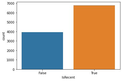
And look at the class distribution:
sns.countplot(train['IsRecent'])
<matplotlib.axes._subplots.AxesSubplot at 0x26bb8bdde80>
Classifying New Papers#
Let’s classify recent papers with k-NN on TF-IDF vectors:
base_knn = Pipeline([
    ('vectorize', TfidfVectorizer(stop_words='english', lowercase=True, max_features=10000)),
    ('class', KNeighborsClassifier(5))
])
base_knn.fit(train['all_text'], train['IsRecent'])
Pipeline(steps=[('vectorize',
                 TfidfVectorizer(max_features=10000, stop_words='english')),
                ('class', KNeighborsClassifier())])
And measure it:
measure(base_knn)
              precision    recall  f1-score   support

       False       0.39      1.00      0.56      1034
        True       0.91      0.01      0.02      1651

    accuracy                           0.39      2685
   macro avg       0.65      0.51      0.29      2685
weighted avg       0.71      0.39      0.23      2685
Tune the Neighborhood#
Let’s tune the neighborhood with a grid search:
tune_knn = Pipeline([
    ('vectorize', TfidfVectorizer(stop_words='english', lowercase=True, max_features=10000)),
    ('class', GridSearchCV(KNeighborsClassifier(), param_grid={
        'n_neighbors': [1, 2, 3, 5, 7, 10]
    }, n_jobs=NJOBS))
])
tune_knn.fit(train['all_text'], train['IsRecent'])
Pipeline(steps=[('vectorize',
                 TfidfVectorizer(max_features=10000, stop_words='english')),
                ('class',
                 GridSearchCV(estimator=KNeighborsClassifier(), n_jobs=8,
                              param_grid={'n_neighbors': [1, 2, 3, 5, 7,
                                                          10]}))])
What did it pick?
tune_knn.named_steps['class'].best_params_
{'n_neighbors': 10}
And measure it:
measure(tune_knn)
              precision    recall  f1-score   support

       False       0.51      0.90      0.65      1034
        True       0.87      0.45      0.60      1651

    accuracy                           0.62      2685
   macro avg       0.69      0.67      0.62      2685
weighted avg       0.73      0.62      0.62      2685
SVD Neighborhood#
Let’s set up SVD-based neighborhood, and use random search to search both the latent feature count and the neighborhood size:
svd_knn_inner = Pipeline([
    ('latent', TruncatedSVD(random_state=rng)),
    ('class', KNeighborsClassifier())
])
svd_knn = Pipeline([
    ('vectorize', TfidfVectorizer(stop_words='english', lowercase=True)),
    ('class', RandomizedSearchCV(svd_knn_inner, param_distributions={
        'latent__n_components': stats.randint(1, 50),
        'class__n_neighbors': stats.randint(1, 25)
    }, n_iter=60, n_jobs=NJOBS, random_state=rng))
])
svd_knn.fit(train['all_text'], train['IsRecent'])
Pipeline(steps=[('vectorize', TfidfVectorizer(stop_words='english')),
                ('class',
                 RandomizedSearchCV(estimator=Pipeline(steps=[('latent',
                                                               TruncatedSVD(random_state=RandomState(MT19937) at 0x26BB86DF140)),
                                                              ('class',
                                                               KNeighborsClassifier())]),
                                    n_iter=60, n_jobs=8,
                                    param_distributions={'class__n_neighbors': <scipy.stats._distn_infrastructure.rv_frozen object at 0x0000026BB8B0BEB0>,
                                                         'latent__n_components': <scipy.stats._distn_infrastructure.rv_frozen object at 0x0000026BB945A070>},
                                    random_state=RandomState(MT19937) at 0x26BB86DF140))])
What parameters did we pick?
svd_knn['class'].best_params_
{'class__n_neighbors': 21, 'latent__n_components': 21}
And measure it on the test data:
measure(svd_knn)
              precision    recall  f1-score   support

       False       0.75      0.47      0.58      1034
        True       0.73      0.90      0.81      1651

    accuracy                           0.74      2685
   macro avg       0.74      0.69      0.69      2685
weighted avg       0.74      0.74      0.72      2685
SVD with scikit-optimize#
Now let’s cross-validate with SciKit-Optimize:
svd_knn_inner = Pipeline([
    ('latent', TruncatedSVD()),
    ('class', KNeighborsClassifier())
])
svd_bayes_knn = Pipeline([
    ('vectorize', TfidfVectorizer(stop_words='english', lowercase=True)),
    ('class', BayesSearchCV(svd_knn_inner, {
        'latent__n_components': (1, 50),
        'class__n_neighbors': (1, 25)
    }, n_jobs=NJOBS, random_state=rng))
])
svd_bayes_knn.fit(train['all_text'], train['IsRecent'])
C:\Users\michaelekstrand\Anaconda3\lib\site-packages\skopt\optimizer\optimizer.py:449: UserWarning: The objective has been evaluated at this point before.
  warnings.warn("The objective has been evaluated "
C:\Users\michaelekstrand\Anaconda3\lib\site-packages\skopt\optimizer\optimizer.py:449: UserWarning: The objective has been evaluated at this point before.
  warnings.warn("The objective has been evaluated "
C:\Users\michaelekstrand\Anaconda3\lib\site-packages\skopt\optimizer\optimizer.py:449: UserWarning: The objective has been evaluated at this point before.
  warnings.warn("The objective has been evaluated "
C:\Users\michaelekstrand\Anaconda3\lib\site-packages\skopt\optimizer\optimizer.py:449: UserWarning: The objective has been evaluated at this point before.
  warnings.warn("The objective has been evaluated "
C:\Users\michaelekstrand\Anaconda3\lib\site-packages\skopt\optimizer\optimizer.py:449: UserWarning: The objective has been evaluated at this point before.
  warnings.warn("The objective has been evaluated "
C:\Users\michaelekstrand\Anaconda3\lib\site-packages\skopt\optimizer\optimizer.py:449: UserWarning: The objective has been evaluated at this point before.
  warnings.warn("The objective has been evaluated "
Pipeline(steps=[('vectorize', TfidfVectorizer(stop_words='english')),
                ('class',
                 BayesSearchCV(estimator=Pipeline(steps=[('latent',
                                                          TruncatedSVD()),
                                                         ('class',
                                                          KNeighborsClassifier())]),
                               n_jobs=8,
                               random_state=RandomState(MT19937) at 0x26BB86DF140,
                               search_spaces={'class__n_neighbors': (1, 25),
                                              'latent__n_components': (1,
                                                                       50)}))])
What parameters did we pick?
svd_bayes_knn['class'].best_params_
OrderedDict([('class__n_neighbors', 25), ('latent__n_components', 20)])
And measure it:
measure(svd_bayes_knn)
              precision    recall  f1-score   support

       False       0.74      0.43      0.55      1034
        True       0.72      0.91      0.80      1651

    accuracy                           0.72      2685
   macro avg       0.73      0.67      0.67      2685
weighted avg       0.73      0.72      0.70      2685
Naive Bayes#
Let’s give the Naive Bayes classifier a whirl:
nb = Pipeline([
    ('vectorize', TfidfVectorizer(stop_words='english', lowercase=True, max_features=10000)),
    ('class', MultinomialNB())
])
nb.fit(train['all_text'], train['IsRecent'])
Pipeline(steps=[('vectorize',
                 TfidfVectorizer(max_features=10000, stop_words='english')),
                ('class', MultinomialNB())])
measure(nb)
              precision    recall  f1-score   support

       False       0.89      0.50      0.64      1034
        True       0.75      0.96      0.85      1651

    accuracy                           0.78      2685
   macro avg       0.82      0.73      0.74      2685
weighted avg       0.81      0.78      0.77      2685
Summary Accuracy#
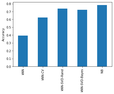
What does our test accuracy look like for our various classifiers?
models = {
    'kNN': base_knn,
    'kNN-CV': tune_knn,
    'kNN-SVD-Rand': svd_knn,
    'kNN-SVD-Bayes': svd_bayes_knn,
    'NB': nb
}
all_preds = pd.DataFrame()
for name, model in models.items():
    all_preds[name] = model.predict(test['all_text'])
acc = all_preds.apply(lambda ds: accuracy_score(test['IsRecent'], ds))
acc
kNN              0.391806
kNN-CV           0.623836
kNN-SVD-Rand     0.735940
kNN-SVD-Bayes    0.724022
NB               0.783240
dtype: float64
acc.plot.bar()
plt.ylabel('Accuracy')
plt.show()