Magic Numbers

Throughout this course, we’ve seen a few different numbers that may appear to be “magic”. This notebook attempts to explain where some of them come from.

Setup

Let’s load a few modules so we can run code usefully.

import pandas as pd
import numpy as np
from scipy import stats
import seaborn as sns
import matplotlib.pyplot as plt

We’re going to do a little random generation, so let’s initialize an RNG:

rng = np.random.default_rng(20221004)

0.025 and 0.975

We’ve used the numbers 0.025 and 0.975 a few times. These come from the left and right tails of a 95% interval.

If we want to pick the middle 95% of a range, such as a data series, that middle 95% starts at 0.025 (2.5%) and ends at 0.975 (97.5%). We get this from:

\[\begin{split}\begin{align*} 1.0 - 0.95 & = 0.05 \\ 0.05 \div 2 &= 0.025 \\ 1.0 - 0.025 & = 0.975 \end{align*}\end{split}\]

1.96

When we compute the 95% confidence interval, we do this by multiplying the standard error by 1.96. Where does this come from?

Let’s create a standard normal distribution:

norm = stats.norm()

And look at its probability density function:

plt.figure(figsize=(5, 2.5))
xs = np.linspace(-4, 4, 1000)
ys = norm.pdf(xs)
plt.plot(xs, ys)
plt.show()

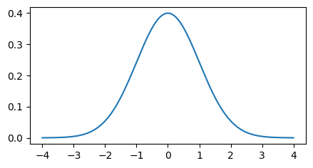
This distribution has \(\mu=0\) and \(\sigma=1\). Suppose we want to to find where the middle 95% of the probability mass is distributed:

plt.figure(figsize=(5, 2.5))
xs = np.linspace(-4, 4, 1000)
ys = norm.pdf(xs)
plt.plot(xs, ys)
plt.fill_between(xs[np.abs(xs) <= 1.96], ys[np.abs(xs) <= 1.96], 0, color='lightblue')
plt.show()

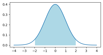
This region extends from -1.96 to 1.96. We can see this by using the normal distribution’s cumulative distribution function:

norm.cdf(-1.96)

0.024997895148220435

That’s 0.025, the number we derived above for the left tail from the central 95% of mass. Let’s see 1.96:

norm.cdf(1.96)

0.9750021048517795

0.975 should look familiar. Now, we can use the formula for the probability mass of an interval to confirm the mass of the interval from -1.96 to 1.96 is 0.95:

norm.cdf(1.96) - norm.cdf(-1.96)

0.950004209703559

We can also derive these values using the inverse CDF, accessible as the ppf method:

norm.ppf([0.025, 0.975])

array([-1.95996398,  1.95996398])

The normal distribution is a scale-location distribution, so the general form of the central 95% interval is \(\mu \pm 1.96 \sigma\).