Reshaping Data#

This notebook discusses operations to reshape data:

Collapsing rows through aggregates
Joining data frames together (basic joins)
Pivoting between wide and long formats

The Selection notebook discussed how to select subsets of rows or columns; these operations will change what the rows and columns are, or add new items.

This notebook uses the “MovieLens + IMDB/RottenTomatoes” data from the HETREC data.

Setup#

First we will import our modules:

import numpy as np
import pandas as pd
import matplotlib.pyplot as plt
import seaborn as sns

Then import the HETREC MovieLens data. A few notes:

Tab-separated data
Not UTF-8 - latin-1 encoding seems to work
Missing data encoded as \N (there’s a good chance that what we have is a PostgreSQL data dump!)

Movies#

movies = pd.read_csv('hetrec2011-ml/movies.dat', delimiter='\t', encoding='latin1', na_values=['\\N'])
movies.head()

	id	title	imdbID	spanishTitle	imdbPictureURL	year	rtID	rtAllCriticsRating	rtAllCriticsNumReviews	rtAllCriticsNumFresh	...	rtAllCriticsScore	rtTopCriticsRating	rtTopCriticsNumReviews	rtTopCriticsNumFresh	rtTopCriticsNumRotten	rtTopCriticsScore	rtAudienceRating	rtAudienceNumRatings	rtAudienceScore	rtPictureURL
0	1	Toy story	114709	Toy story (juguetes)	http://ia.media-imdb.com/images/M/MV5BMTMwNDU0...	1995	toy_story	9.0	73.0	73.0	...	100.0	8.5	17.0	17.0	0.0	100.0	3.7	102338.0	81.0	http://content7.flixster.com/movie/10/93/63/10...
1	2	Jumanji	113497	Jumanji	http://ia.media-imdb.com/images/M/MV5BMzM5NjE1...	1995	1068044-jumanji	5.6	28.0	13.0	...	46.0	5.8	5.0	2.0	3.0	40.0	3.2	44587.0	61.0	http://content8.flixster.com/movie/56/79/73/56...
2	3	Grumpy Old Men	107050	Dos viejos gruñones	http://ia.media-imdb.com/images/M/MV5BMTI5MTgy...	1993	grumpy_old_men	5.9	36.0	24.0	...	66.0	7.0	6.0	5.0	1.0	83.0	3.2	10489.0	66.0	http://content6.flixster.com/movie/25/60/25602...
3	4	Waiting to Exhale	114885	Esperando un respiro	http://ia.media-imdb.com/images/M/MV5BMTczMTMy...	1995	waiting_to_exhale	5.6	25.0	14.0	...	56.0	5.5	11.0	5.0	6.0	45.0	3.3	5666.0	79.0	http://content9.flixster.com/movie/10/94/17/10...
4	5	Father of the Bride Part II	113041	Vuelve el padre de la novia (Ahora también abu...	http://ia.media-imdb.com/images/M/MV5BMTg1NDc2...	1995	father_of_the_bride_part_ii	5.3	19.0	9.0	...	47.0	5.4	5.0	1.0	4.0	20.0	3.0	13761.0	64.0	http://content8.flixster.com/movie/25/54/25542...

5 rows × 21 columns

movies.info()

<class 'pandas.core.frame.DataFrame'>
RangeIndex: 10197 entries, 0 to 10196
Data columns (total 21 columns):
 #   Column                  Non-Null Count  Dtype  
---  ------                  --------------  -----  
 id                      10197 non-null  int64  
 title                   10197 non-null  object 
 imdbID                  10197 non-null  int64  
 spanishTitle            10197 non-null  object 
 imdbPictureURL          10016 non-null  object 
 year                    10197 non-null  int64  
 rtID                    9886 non-null   object 
 rtAllCriticsRating      9967 non-null   float64
 rtAllCriticsNumReviews  9967 non-null   float64
 rtAllCriticsNumFresh    9967 non-null   float64
rtAllCriticsNumRotten   9967 non-null   float64
rtAllCriticsScore       9967 non-null   float64
rtTopCriticsRating      9967 non-null   float64
rtTopCriticsNumReviews  9967 non-null   float64
rtTopCriticsNumFresh    9967 non-null   float64
rtTopCriticsNumRotten   9967 non-null   float64
rtTopCriticsScore       9967 non-null   float64
rtAudienceRating        9967 non-null   float64
rtAudienceNumRatings    9967 non-null   float64
rtAudienceScore         9967 non-null   float64
rtPictureURL            9967 non-null   object 
dtypes: float64(13), int64(3), object(5)
memory usage: 1.6+ MB

Movie Info#

movie_genres = pd.read_csv('hetrec2011-ml/movie_genres.dat', delimiter='\t', encoding='latin1')
movie_genres.head()

	movieID	genre
0	1	Adventure
1	1	Animation
2	1	Children
3	1	Comedy
4	1	Fantasy

movie_tags = pd.read_csv('hetrec2011-ml/movie_tags.dat', delimiter='\t', encoding='latin1')
movie_tags.head()

	movieID	tagID	tagWeight
0	1	7	1
1	1	13	3
2	1	25	3
3	1	55	3
4	1	60	1

tags = pd.read_csv('hetrec2011-ml/tags.dat', delimiter='\t', encoding='latin1')
tags.head()

	id	value
0	1	earth
1	2	police
2	3	boxing
3	4	painter
4	5	whale

Ratings#

ratings = pd.read_csv('hetrec2011-ml/user_ratedmovies-timestamps.dat', delimiter='\t', encoding='latin1')
ratings.head()

	userID	movieID	rating	timestamp
0	75	3	1.0	1162160236000
1	75	32	4.5	1162160624000
2	75	110	4.0	1162161008000
3	75	160	2.0	1162160212000
4	75	163	4.0	1162160970000

Grouping and Aggregating#

The group and aggregate operations allow us to collapse multiple rows, that share a common value in one or more columns (the grouping key), into a single row. There are three pieces of a group-aggregate operation:

The grouping key — one or more columns that are used to identify which rows are in the same group
The column(s) to aggregate
The aggregate function(s) to apply

A group/aggregate operation transforms a data frames using thes columns as follows:

Each unique combination of values in the grouping key becomes one row. If the grouping key is one column, this means each distinct value of the grouping column will yield one row in the final results.
The columns to aggregate are collapsed into a single value using the specified aggregate function(s).
Other columns are ignored and do not appear in the output.

Aggregate to Series#

If we have: a data frame
And we have: a column identifying each observation’s group membership
And we want: a series with an entry for each group, whose value is an aggregate function of another column
Then we can: use groupby with one column and the aggregate function.

For example, if we want to find the timestamp of the first rating for each movie, we can group the ratings table by movieID and take the min of the timestamp column:

ratings.groupby('movieID')['timestamp'].min()

movieID
       876894948000
       891835167000
       931525286000
       951680805000
       874593700000
             ...      
  1230851753000
  1230918649000
  1231028759000
  1231061731000
  1231034528000
Name: timestamp, Length: 10109, dtype: int64

This breaks down into a few pieces. The groupby method returns a group-by object:

ratings.groupby('movieID')

<pandas.core.groupby.generic.DataFrameGroupBy object at 0x00000270239AA7F0>

The DataFrameGroupBy is a iterable over (key, df) tuples, where key is a single value of the grouping key, and df is a data frame containing the group’s data (the next function gets the next value of an iterable):

next(iter(ratings.groupby('movieID')))

(1,
         userID  movieID  rating      timestamp
 556        170        1     3.0  1162208198000
 639        175        1     4.0  1133674606000
 915        190        1     4.5  1057778398000
 1211       267        1     2.5  1084284499000
 1643       325        1     4.0  1134939391000
 ...        ...      ...     ...            ...
 850646   71420        1     5.0   948256089000
 852838   71483        1     4.0  1035837220000
 853507   71497        1     5.0  1188256917000
 853757   71509        1     4.0  1018636872000
 855327   71529        1     4.5  1162098801000
 
 [1263 rows x 4 columns])

The column selection yields a SeriesGroupBy, which is a group-by for a series instead of a frame:

ratings.groupby('movieID')['timestamp']

<pandas.core.groupby.generic.SeriesGroupBy object at 0x00000270239AAD30>

Finally, calling min on this will apply the min function to each group, and put the results together into a series.

Multiple Aggregates#

If we have: a data frame
And we have: a column identifying each observation’s group membership
And we want: a data frame with an entry for each group, with a column for each of one or more aggregate functions of a column
Then we can: use groupby with one column and the .agg method with aggregate function names

For example, if we want to find the timestamp of the first rating and last ratings for each movie, we can group the ratings table by movieID and take the min and max of the timestamp column:

ratings.groupby('movieID')['timestamp'].agg(['min', 'max'])

	min	max
movieID
1	876894948000	1231030405000
2	891835167000	1231030891000
3	931525286000	1231099805000
4	951680805000	1229214105000
5	874593700000	1230915209000
...	...	...
65088	1230851753000	1230851753000
65091	1230918649000	1230918649000
65126	1231028759000	1231097168000
65130	1231061731000	1231061731000
65133	1231034528000	1231129793000

10109 rows × 2 columns

Note that in both cases, the resulting frame or series is indexed by the grouping column.

Practice: compute the mean and count of the ratings for each movie

Counting Values#

There’s a useful special case of grouped aggregation - counting how many times each distinct value in a column appears.

If we have: a series
And we want: a series whose index keys are the values of the original series, and whose values are the number of times each value appeared in the original series
Then we can: use the value_counts method:

ratings['rating'].value_counts()

0    215773
0    155918
5    150582
5     88652
0     71680
5     62454
0     57188
0     21535
5     18328
5     13488
Name: rating, dtype: int64

We can also sort the results with the sort_index method:

ratings['rating'].value_counts().sort_index()

5     13488
0     21535
5     18328
0     57188
5     62454
0    155918
5    150582
0    215773
5     88652
0     71680
Name: rating, dtype: int64

sort_index applies to both series and data frames.

Multiple Columns#

We can also compute an aggregate over multiple columns at the same time. For example, if we want to look at the mean critic and audience scores of movies over time, we can group movies by year and take the mean of multiple columns.

If we have: a data frame
And we have: one or more columns identifying group membership
And we want: a data frame with the same aggregate computed over all other columns in the frame
Then we can: apply groupby and the aggregate function without selecting columns.

We’re first going to select and rename columns, like we did at the end of the Selection notebook.

movie_scores = movies.set_index('id')[['year', 'rtAllCriticsRating', 'rtTopCriticsRating', 'rtAudienceRating']].rename(columns={
    'rtAllCriticsRating': 'All Critics',
    'rtTopCriticsRating': 'Top Critics',
    'rtAudienceRating': 'Audience'
})
movie_scores

	year	All Critics	Top Critics	Audience
id
1	1995	9.0	8.5	3.7
2	1995	5.6	5.8	3.2
3	1993	5.9	7.0	3.2
4	1995	5.6	5.5	3.3
5	1995	5.3	5.4	3.0
...	...	...	...	...
65088	2008	4.4	4.7	3.5
65091	1934	7.0	0.0	3.7
65126	2008	5.6	4.9	3.3
65130	2008	6.7	6.9	3.5
65133	1999	0.0	0.0	0.0

10197 rows × 4 columns

Now we’re going to do the group-by operation:

year_scores = movie_scores.groupby('year').mean()
year_scores

	All Critics	Top Critics	Audience
year
1903	7.600000	0.000000	0.000000
1915	8.000000	0.000000	3.300000
1916	7.800000	0.000000	3.800000
1917	0.000000	0.000000	0.000000
1918	0.000000	0.000000	0.000000
...	...	...	...
2007	5.141278	4.769042	3.062162
2008	4.699357	4.383280	2.853698
2009	4.850000	4.700000	3.192308
2010	0.000000	0.000000	0.000000
2011	0.000000	0.000000	0.000000

98 rows × 3 columns

There are two other equivalents to this operation. First, the agg function can take one name instead of a list:

movie_scores.groupby('year').agg('mean')

	All Critics	Top Critics	Audience
year
1903	7.600000	0.000000	0.000000
1915	8.000000	0.000000	3.300000
1916	7.800000	0.000000	3.800000
1917	0.000000	0.000000	0.000000
1918	0.000000	0.000000	0.000000
...	...	...	...
2007	5.141278	4.769042	3.062162
2008	4.699357	4.383280	2.853698
2009	4.850000	4.700000	3.192308
2010	0.000000	0.000000	0.000000
2011	0.000000	0.000000	0.000000

98 rows × 3 columns

Second, the agg function can actually take a function as its argument:

movie_scores.groupby('year').agg(np.mean)

	All Critics	Top Critics	Audience
year
1903	7.600000	0.000000	0.000000
1915	8.000000	0.000000	3.300000
1916	7.800000	0.000000	3.800000
1917	0.000000	0.000000	0.000000
1918	0.000000	0.000000	0.000000
...	...	...	...
2007	5.141278	4.769042	3.062162
2008	4.699357	4.383280	2.853698
2009	4.850000	4.700000	3.192308
2010	0.000000	0.000000	0.000000
2011	0.000000	0.000000	0.000000

98 rows × 3 columns

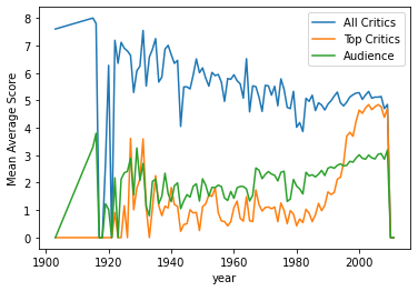
No matter which method we used, we can then quickly do a line plot, which will default to plotting each column as a different colored line, with the index on the x axis:

year_scores.plot.line()
plt.ylabel('Mean Average Score')
plt.show()

Other Grouping Modes#

There are a couple of other ways you can use groupby and aggregates:

Select multiple columns from the data frame grouper, by using a list of columns.
Apply a different aggregate to each function by passing a dictionary to agg.
Apply multiple aggregates to multiple columns by passing a list to agg and selecting a list of columns. The resulting data frame has a hierarchical index for its columns, which is honestly a little annoying to actually use.
Group by multiple columns, resulting in a hierarchical index for the rows

Experiment with these on your own!

Note: if you use multiple columns, and one or more of the columns of the frame is a Categorical, groupby will produce a row for each possible value, even if one is never observed for that combination of the other grouping keys. To turn this off, pass the observed=True option to groupby.

Joining Frames#

We can join two frames together based on common values of one or more of their columns, possibly using indexes as well.

The simplest way to join two frames without any indexes is with pd.merge.

Column Join#

If we have: two data frames with at least one column in common
And we want: a data frame with rows based on matching the column values
Then we can: use pd.merge to join the frames.

For example, to combine genres with titles:

pd.merge(movies[['id', 'title']].rename(columns={'id': 'movieID'}),
         movie_genres, on='movieID')

	movieID	title	genre
0	1	Toy story	Adventure
1	1	Toy story	Animation
2	1	Toy story	Children
3	1	Toy story	Comedy
4	1	Toy story	Fantasy
...	...	...	...
20804	65126	Choke	Comedy
20805	65126	Choke	Drama
20806	65130	Revolutionary Road	Drama
20807	65130	Revolutionary Road	Romance
20808	65133	Blackadder Back & Forth	Comedy

20809 rows × 3 columns

If there is more than one row in one table with a match for a value in the other table, it duplicates the other row. So we can see that “Toy story” is duplicated, once for each genre it appears in.

Pull out the selection & rename on movies into a new cell for practice, and to see what it does.

Column/Index Join#

The join method can do index-index and column-index joins.

If we have: a data frame
And we have: another data frame whose index is values appearing in a column of the first frame
And we want: a frame that merges the two frames by matching column values in the first with the index keys of the second
Then we can: use .join with the on option.

To set this up, we want something with a suitable index. Let’s create a frame that has mean & count of MovieLens user ratings:

movie_stats = ratings.groupby('movieID')['rating'].agg(['mean', 'count'])
movie_stats = movie_stats.rename(columns={'mean': 'MeanRating', 'count': 'RatingCount'})
movie_stats

	MeanRating	RatingCount
movieID
1	3.735154	1263
2	2.976471	765
3	2.873016	252
4	2.577778	45
5	2.753333	225
...	...	...
65088	3.500000	1
65091	4.000000	1
65126	3.250000	2
65130	2.500000	1
65133	4.000000	3

10109 rows × 2 columns

This frame is indexed by movieID. Let’s combine that with movie title & year info:

movies[['id', 'title', 'year']].join(movie_stats, on='id')

	id	title	year	MeanRating	RatingCount
0	1	Toy story	1995	3.735154	1263.0
1	2	Jumanji	1995	2.976471	765.0
2	3	Grumpy Old Men	1993	2.873016	252.0
3	4	Waiting to Exhale	1995	2.577778	45.0
4	5	Father of the Bride Part II	1995	2.753333	225.0
...	...	...	...	...	...
10192	65088	Bedtime Stories	2008	3.500000	1.0
10193	65091	Manhattan Melodrama	1934	4.000000	1.0
10194	65126	Choke	2008	3.250000	2.0
10195	65130	Revolutionary Road	2008	2.500000	1.0
10196	65133	Blackadder Back & Forth	1999	4.000000	3.0

10197 rows × 5 columns

Note that we used the id column, which is in the movies table, as the on option. Join automatically matches it with the index in movie_stats.

Index/Index Join#

Let’s now see an index-index join.

If we have: two data frames with matching indexes
And we want: a frame that merges the two frames matching their index values
Then we can: use .join with no extra options.

Remember that set_index will set an index on the movies frame:

movies.set_index('id')

	title	imdbID	spanishTitle	imdbPictureURL	year	rtID	rtAllCriticsRating	rtAllCriticsNumReviews	rtAllCriticsNumFresh	rtAllCriticsNumRotten	rtAllCriticsScore	rtTopCriticsRating	rtTopCriticsNumReviews	rtTopCriticsNumFresh	rtTopCriticsNumRotten	rtTopCriticsScore	rtAudienceRating	rtAudienceNumRatings	rtAudienceScore	rtPictureURL
id
1	Toy story	114709	Toy story (juguetes)	http://ia.media-imdb.com/images/M/MV5BMTMwNDU0...	1995	toy_story	9.0	73.0	73.0	0.0	100.0	8.5	17.0	17.0	0.0	100.0	3.7	102338.0	81.0	http://content7.flixster.com/movie/10/93/63/10...
2	Jumanji	113497	Jumanji	http://ia.media-imdb.com/images/M/MV5BMzM5NjE1...	1995	1068044-jumanji	5.6	28.0	13.0	15.0	46.0	5.8	5.0	2.0	3.0	40.0	3.2	44587.0	61.0	http://content8.flixster.com/movie/56/79/73/56...
3	Grumpy Old Men	107050	Dos viejos gruñones	http://ia.media-imdb.com/images/M/MV5BMTI5MTgy...	1993	grumpy_old_men	5.9	36.0	24.0	12.0	66.0	7.0	6.0	5.0	1.0	83.0	3.2	10489.0	66.0	http://content6.flixster.com/movie/25/60/25602...
4	Waiting to Exhale	114885	Esperando un respiro	http://ia.media-imdb.com/images/M/MV5BMTczMTMy...	1995	waiting_to_exhale	5.6	25.0	14.0	11.0	56.0	5.5	11.0	5.0	6.0	45.0	3.3	5666.0	79.0	http://content9.flixster.com/movie/10/94/17/10...
5	Father of the Bride Part II	113041	Vuelve el padre de la novia (Ahora también abu...	http://ia.media-imdb.com/images/M/MV5BMTg1NDc2...	1995	father_of_the_bride_part_ii	5.3	19.0	9.0	10.0	47.0	5.4	5.0	1.0	4.0	20.0	3.0	13761.0	64.0	http://content8.flixster.com/movie/25/54/25542...
...	...	...	...	...	...	...	...	...	...	...	...	...	...	...	...	...	...	...	...	...
65088	Bedtime Stories	960731	Más allá de los sueños	http://ia.media-imdb.com/images/M/MV5BMjA5Njk5...	2008	bedtime_stories	4.4	104.0	26.0	78.0	25.0	4.7	26.0	6.0	20.0	23.0	3.5	108877.0	63.0	http://content6.flixster.com/movie/10/94/33/10...
65091	Manhattan Melodrama	25464	El enemigo público número 1	http://ia.media-imdb.com/images/M/MV5BMTUyODE3...	1934	manhattan_melodrama	7.0	12.0	10.0	2.0	83.0	0.0	4.0	2.0	2.0	50.0	3.7	344.0	71.0	http://content9.flixster.com/movie/66/44/64/66...
65126	Choke	1024715	Choke	http://ia.media-imdb.com/images/M/MV5BMTMxMDI4...	2008	choke	5.6	135.0	73.0	62.0	54.0	4.9	26.0	8.0	18.0	30.0	3.3	13893.0	55.0	http://content6.flixster.com/movie/10/85/09/10...
65130	Revolutionary Road	959337	Revolutionary Road	http://ia.media-imdb.com/images/M/MV5BMTI2MzY2...	2008	revolutionary_road	6.7	194.0	133.0	61.0	68.0	6.9	36.0	25.0	11.0	69.0	3.5	46044.0	70.0	http://content8.flixster.com/movie/10/88/40/10...
65133	Blackadder Back & Forth	212579	Blackadder Back & Forth	http://ia.media-imdb.com/images/M/MV5BMjA5MjU4...	1999	blackadder-back-forth	0.0	0.0	0.0	0.0	0.0	0.0	0.0	0.0	0.0	0.0	0.0	0.0	0.0	http://content7.flixster.com/movie/34/10/69/34...

10197 rows × 20 columns

So we’ll set the index, pick a couple columns, and join with movie stats:

movies.set_index('id')[['title', 'year']].join(movie_stats)

	title	year	MeanRating	RatingCount
id
1	Toy story	1995	3.735154	1263.0
2	Jumanji	1995	2.976471	765.0
3	Grumpy Old Men	1993	2.873016	252.0
4	Waiting to Exhale	1995	2.577778	45.0
5	Father of the Bride Part II	1995	2.753333	225.0
...	...	...	...	...
65088	Bedtime Stories	2008	3.500000	1.0
65091	Manhattan Melodrama	1934	4.000000	1.0
65126	Choke	2008	3.250000	2.0
65130	Revolutionary Road	2008	2.500000	1.0
65133	Blackadder Back & Forth	1999	4.000000	3.0

10197 rows × 4 columns

This has the same result.

Join Types#

There are multiple types of joins. The types of Pandas joins correspond to SQL join types, if you are familiar with those.

We refer to the frames as left and right. These correspond to positions in the functions as follows:

pd.merge(left, right)
left.join(right)

An inner join requires a match to appear in both frames. If there is a row in one frame whose join column value has no match in the other frame, the row is excluded. This applies to both frames.
A left join includes every row in the left-hand frame at least once; if there is a left-hand row with no match in the right-hand frame, one copy is included with missing values for all of the right-hand columns. Right-hand rows with no matches in the left frame are excluded.
A right join is the reverse of a left join: it includes every value in the right-hand frame at least once.
An outer join includes every row from both frames at least once.

pd.merge defaults to an inner join, and left.join(right) defaults to a left join. Both take a how= option to change the merge type.

Join Tips#

The join I find myself using most frequently is a column-index join. I also usually join on a single column, although multiple-column joins are very well-supported.

Tall and Wide#

As discussed in the video, data comes in tall and wide formats. If we observations of multiple variables for something, it can be in either format:

In wide format, each variable is a column
In tall (or long) format, each variable produces a new row; there is a column for the variable name and another for the value

We can convert back and forth between them.

Tall to Wide#

The pivot function converts tall data to wide data.

First, let’s make some tall data. The movie-tags table has the tags that apply to each movie, along with their weight: how important that tag is. Let’s look (joining to tag to get the tag names):

movie_tags.join(tags.set_index('id'), on='tagID')

	movieID	tagID	tagWeight	value
0	1	7	1	funny
1	1	13	3	time travel
2	1	25	3	tim allen
3	1	55	3	comedy
4	1	60	1	fun
...	...	...	...	...
51790	65037	792	1	autism
51791	65037	2214	1	internet
51792	65126	5281	1	based on book
51793	65126	13168	1	chuck palahniuk
51794	65130	2924	1	toplist08

51795 rows × 4 columns

value is a funny name, and once we have name we don’t need tag ID, so let’s clean up these columns:

movie_tag_weights = movie_tags.join(tags.set_index('id'), on='tagID')
movie_tag_weights = movie_tag_weights[['movieID', 'value', 'tagWeight']]
movie_tag_weights = movie_tag_weights.rename(columns={
    'value': 'tag',
    'tagWeight': 'weight'
})
movie_tag_weights

	movieID	tag	weight
0	1	funny	1
1	1	time travel	3
2	1	tim allen	3
3	1	comedy	3
4	1	fun	1
...	...	...	...
51790	65037	autism	1
51791	65037	internet	1
51792	65126	based on book	1
51793	65126	chuck palahniuk	1
51794	65130	toplist08	1

51795 rows × 3 columns

This is in tall format: for each movie, we have a row for each tag with its weight.

If we want to turn this into a (very!) wide table, with a column for each tag, we can use pivot.

If we have: a data frame in tall format (one column has variable names, and another their values)
And we want: the same data in wide format (variables split out into columns)
Then we can: use pivot to pivot the tall data into wide format:

mtw_wide = movie_tag_weights.pivot('movieID', 'tag', 'weight')
mtw_wide

tag	(s)vcd	007 (series)	15th century	16mm	16th century	17th century	1800s	1890s	18th century	1900s	...	zeppelin	zero mostel	zibri studio	zim	ziyi zhang	zombie	zombie movie	zombies	zoo	zooey deschanel
movieID
1	NaN	NaN	NaN	NaN	NaN	NaN	NaN	NaN	NaN	NaN	...	NaN	NaN	NaN	NaN	NaN	NaN	NaN	NaN	NaN	NaN
2	NaN	NaN	NaN	NaN	NaN	NaN	NaN	NaN	NaN	NaN	...	NaN	NaN	NaN	NaN	NaN	NaN	NaN	NaN	NaN	NaN
3	NaN	NaN	NaN	NaN	NaN	NaN	NaN	NaN	NaN	NaN	...	NaN	NaN	NaN	NaN	NaN	NaN	NaN	NaN	NaN	NaN
5	NaN	NaN	NaN	NaN	NaN	NaN	NaN	NaN	NaN	NaN	...	NaN	NaN	NaN	NaN	NaN	NaN	NaN	NaN	NaN	NaN
6	NaN	NaN	NaN	NaN	NaN	NaN	NaN	NaN	NaN	NaN	...	NaN	NaN	NaN	NaN	NaN	NaN	NaN	NaN	NaN	NaN
...	...	...	...	...	...	...	...	...	...	...	...	...	...	...	...	...	...	...	...	...	...
64993	NaN	NaN	NaN	NaN	NaN	NaN	NaN	NaN	NaN	NaN	...	NaN	NaN	NaN	NaN	NaN	NaN	NaN	NaN	NaN	NaN
65006	NaN	NaN	NaN	NaN	NaN	NaN	NaN	NaN	NaN	NaN	...	NaN	NaN	NaN	NaN	NaN	NaN	NaN	NaN	NaN	NaN
65037	NaN	NaN	NaN	NaN	NaN	NaN	NaN	NaN	NaN	NaN	...	NaN	NaN	NaN	NaN	NaN	NaN	NaN	NaN	NaN	NaN
65126	NaN	NaN	NaN	NaN	NaN	NaN	NaN	NaN	NaN	NaN	...	NaN	NaN	NaN	NaN	NaN	NaN	NaN	NaN	NaN	NaN
65130	NaN	NaN	NaN	NaN	NaN	NaN	NaN	NaN	NaN	NaN	...	NaN	NaN	NaN	NaN	NaN	NaN	NaN	NaN	NaN	NaN

7155 rows × 5297 columns

We see a lot of missing values (NaN). The describe method on a data frame will describe all the columns, which will include counting the values. Let’s see it:

mtw_desc = mtw_wide.describe()
mtw_desc

tag	(s)vcd	007 (series)	15th century	16mm	16th century	17th century	1800s	1890s	18th century	1900s	...	zeppelin	zero mostel	zibri studio	zim	ziyi zhang	zombie	zombie movie	zombies	zoo	zooey deschanel
count	31.000000	23.000000	2.0	5.0	6.0	10.000000	2.0	4.0	12.000000	7.000000	...	2.0	2.0	9.000000	7.0	2.0	25.00000	3.0	43.000000	2.0	2.0
mean	1.032258	1.043478	1.0	1.0	1.0	1.300000	1.0	1.0	1.583333	1.142857	...	1.0	1.0	1.111111	1.0	1.0	1.52000	2.0	3.465116	1.0	1.0
std	0.179605	0.208514	0.0	0.0	0.0	0.483046	0.0	0.0	0.996205	0.377964	...	0.0	0.0	0.333333	0.0	0.0	0.87178	1.0	3.607854	0.0	0.0
min	1.000000	1.000000	1.0	1.0	1.0	1.000000	1.0	1.0	1.000000	1.000000	...	1.0	1.0	1.000000	1.0	1.0	1.00000	1.0	1.000000	1.0	1.0
25%	1.000000	1.000000	1.0	1.0	1.0	1.000000	1.0	1.0	1.000000	1.000000	...	1.0	1.0	1.000000	1.0	1.0	1.00000	1.5	1.000000	1.0	1.0
50%	1.000000	1.000000	1.0	1.0	1.0	1.000000	1.0	1.0	1.000000	1.000000	...	1.0	1.0	1.000000	1.0	1.0	1.00000	2.0	2.000000	1.0	1.0
75%	1.000000	1.000000	1.0	1.0	1.0	1.750000	1.0	1.0	2.000000	1.000000	...	1.0	1.0	1.000000	1.0	1.0	2.00000	2.5	5.000000	1.0	1.0
max	2.000000	2.000000	1.0	1.0	1.0	2.000000	1.0	1.0	4.000000	2.000000	...	1.0	1.0	2.000000	1.0	1.0	4.00000	3.0	19.000000	1.0	1.0

8 rows × 5297 columns

That might look better if we switch columns and rows:

mtw_desc.T

	count	mean	std	min	25%	50%	75%	max
tag
(s)vcd	31.0	1.032258	0.179605	1.0	1.0	1.0	1.0	2.0
007 (series)	23.0	1.043478	0.208514	1.0	1.0	1.0	1.0	2.0
15th century	2.0	1.000000	0.000000	1.0	1.0	1.0	1.0	1.0
16mm	5.0	1.000000	0.000000	1.0	1.0	1.0	1.0	1.0
16th century	6.0	1.000000	0.000000	1.0	1.0	1.0	1.0	1.0
...	...	...	...	...	...	...	...	...
zombie	25.0	1.520000	0.871780	1.0	1.0	1.0	2.0	4.0
zombie movie	3.0	2.000000	1.000000	1.0	1.5	2.0	2.5	3.0
zombies	43.0	3.465116	3.607854	1.0	1.0	2.0	5.0	19.0
zoo	2.0	1.000000	0.000000	1.0	1.0	1.0	1.0	1.0
zooey deschanel	2.0	1.000000	0.000000	1.0	1.0	1.0	1.0	1.0

5297 rows × 8 columns

Ok isn’t that kinda cool?

Stacking Frames#

Joins let us combine by merging on values, but sometimes we want to stack data frames on top of each other. The concat Pandas function concatenates a list (or other iterable) of data frames. For example, to simulate a melt of the two critic rating columns:

movie_top_rates = movies[['id', 'rtTopCriticsRating']].rename(columns={'rtTopCriticsRating': 'rating'})
movie_top_rates['source'] = 'Top Critics'
movie_all_rates = movies[['id', 'rtAllCriticsRating']].rename(columns={'rtAllCriticsRating': 'rating'})
movie_all_rates['source'] = 'All Critics'

movie_rates = pd.concat([movie_top_rates, movie_all_rates], ignore_index=True)
movie_rates

	id	rating	source
0	1	8.5	Top Critics
1	2	5.8	Top Critics
2	3	7.0	Top Critics
3	4	5.5	Top Critics
4	5	5.4	Top Critics
...	...	...	...
20389	65088	4.4	All Critics
20390	65091	7.0	All Critics
20391	65126	5.6	All Critics
20392	65130	6.7	All Critics
20393	65133	0.0	All Critics

20394 rows × 3 columns

The ignore_index=True option causes pd.concat to throw away the indexes and make a new RangeIndex. This is fine because the indexes don’t contain any useful information.

We can also concatenate with the index; this is most useful when the frames have disjoint indexes, or when we want to add another index level containing the source. We’ll discuss this in the indexing notebook.

Wide to Tall#

What if we want to go the other way? That’s what melt is for.

Remember our movie stats by year?

year_scores

	All Critics	Top Critics	Audience
year
1903	7.600000	0.000000	0.000000
1915	8.000000	0.000000	3.300000
1916	7.800000	0.000000	3.800000
1917	0.000000	0.000000	0.000000
1918	0.000000	0.000000	0.000000
...	...	...	...
2007	5.141278	4.769042	3.062162
2008	4.699357	4.383280	2.853698
2009	4.850000	4.700000	3.192308
2010	0.000000	0.000000	0.000000
2011	0.000000	0.000000	0.000000

98 rows × 3 columns

If we have: a data frame in wide format
And we want: the same data in tall format
Then we can: use the melt method or function.

We first have to reset the index, because melt destroys it:

year_scores.reset_index()

	year	All Critics	Top Critics	Audience
0	1903	7.600000	0.000000	0.000000
1	1915	8.000000	0.000000	3.300000
2	1916	7.800000	0.000000	3.800000
3	1917	0.000000	0.000000	0.000000
4	1918	0.000000	0.000000	0.000000
...	...	...	...	...
93	2007	5.141278	4.769042	3.062162
94	2008	4.699357	4.383280	2.853698
95	2009	4.850000	4.700000	3.192308
96	2010	0.000000	0.000000	0.000000
97	2011	0.000000	0.000000	0.000000

98 rows × 4 columns

That pops the year back out to being a column, so we can pass it as the id_var to melt:

ys_tall = year_scores.reset_index().melt(id_vars='year')
ys_tall

	year	variable	value
0	1903	All Critics	7.600000
1	1915	All Critics	8.000000
2	1916	All Critics	7.800000
3	1917	All Critics	0.000000
4	1918	All Critics	0.000000
...	...	...	...
289	2007	Audience	3.062162
290	2008	Audience	2.853698
291	2009	Audience	3.192308
292	2010	Audience	0.000000
293	2011	Audience	0.000000

294 rows × 3 columns

We can give better names to these things:

ys_tall = year_scores.reset_index().melt(id_vars='year', var_name='Source', value_name='MeanAvgScore')
ys_tall

	year	Source	MeanAvgScore
0	1903	All Critics	7.600000
1	1915	All Critics	8.000000
2	1916	All Critics	7.800000
3	1917	All Critics	0.000000
4	1918	All Critics	0.000000
...	...	...	...
289	2007	Audience	3.062162
290	2008	Audience	2.853698
291	2009	Audience	3.192308
292	2010	Audience	0.000000
293	2011	Audience	0.000000

294 rows × 3 columns

This is useful for plotting - year is the x axis, score, the y, and source the color or hue:

sns.lineplot('year', 'MeanAvgScore', hue='Source', data=ys_tall)

<matplotlib.axes._subplots.AxesSubplot at 0x270245c6460>

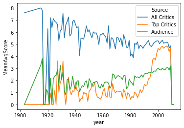
In practice, setting up plots is one of my most frequent use cases for melt. The Pandas defaults we saw earlier are useful, but this give us much more control.

CS 533 Fall 2022

Reshaping Data

Contents

Reshaping Data#

Setup#

Movies#

Movie Info#

Ratings#

Grouping and Aggregating#

Aggregate to Series#

Multiple Aggregates#

Counting Values#

Multiple Columns#

Other Grouping Modes#

Joining Frames#

Column Join#

Column/Index Join#

Index/Index Join#

Join Types#

Join Tips#

Tall and Wide#

Tall to Wide#

Stacking Frames#

Wide to Tall#