Sampling and Testing the Penguins
Contents
Sampling and Testing the Penguins#
This notebook uses the Palmer Penguins data to demonstrate confidence intervals and two-sample hypothesis tests, both using parametric methods and the bootstrap.
Our question: What are the average values of various penguin dimensions (bill length and depth, flipper length, and body mass)? Do these dimensions differ between penguin species?
Setup#
Python modules:
import numpy as np
import pandas as pd
import scipy.stats as sps
import statsmodels.api as sm
import matplotlib.pyplot as plt
import seaborn as sns
Set up a random number generator:
rng = np.random.default_rng(20200913)
Load the Penguin data:
penguins = pd.read_csv('../data/penguins.csv')
penguins.head()
| species | island | bill_length_mm | bill_depth_mm | flipper_length_mm | body_mass_g | sex | year | |
|---|---|---|---|---|---|---|---|---|
| 0 | Adelie | Torgersen | 39.1 | 18.7 | 181.0 | 3750.0 | male | 2007 |
| 1 | Adelie | Torgersen | 39.5 | 17.4 | 186.0 | 3800.0 | female | 2007 |
| 2 | Adelie | Torgersen | 40.3 | 18.0 | 195.0 | 3250.0 | female | 2007 |
| 3 | Adelie | Torgersen | NaN | NaN | NaN | NaN | NaN | 2007 |
| 4 | Adelie | Torgersen | 36.7 | 19.3 | 193.0 | 3450.0 | female | 2007 |
Some of these names are cumbersome to deal with. I’m going to give them shorter names:
penguins.rename(columns={
    'bill_length_mm': 'BillLength',
    'bill_depth_mm': 'BillDepth',
    'flipper_length_mm': 'FlipperLength',
    'body_mass_g': 'Mass'
}, inplace=True)
A few things will be eaiser if we also split out penguins by species:
chinstraps = penguins[penguins['species'] == 'Chinstrap']
chinstraps.head()
| species | island | BillLength | BillDepth | FlipperLength | Mass | sex | year | |
|---|---|---|---|---|---|---|---|---|
| 276 | Chinstrap | Dream | 46.5 | 17.9 | 192.0 | 3500.0 | female | 2007 |
| 277 | Chinstrap | Dream | 50.0 | 19.5 | 196.0 | 3900.0 | male | 2007 |
| 278 | Chinstrap | Dream | 51.3 | 19.2 | 193.0 | 3650.0 | male | 2007 |
| 279 | Chinstrap | Dream | 45.4 | 18.7 | 188.0 | 3525.0 | female | 2007 |
| 280 | Chinstrap | Dream | 52.7 | 19.8 | 197.0 | 3725.0 | male | 2007 |
adelies = penguins[penguins['species'] == 'Adelie']
gentoos = penguins[penguins['species'] == 'Gentoo']
That’s all we need right now!
Confidence Intervals#
Remember that \(s/\sqrt{n}\) is the standard error of the mean. The SciPy sem function computes the standard error of the mean. We can multiply this by 1.96 to get the distance between the sample mean and the edge of the confidence interval.
So let’s write a function that returns the 95% CI of the mean of some data:
def mean_ci95(xs):
    mean = np.mean(xs)
    err = sps.sem(xs)
    width = 1.96 * err
    return mean - width, mean + width
Warmup: Chinstrap Flippers#
As a warmup, let’s compute confidence intervals for the chinstrap flipper length. We will do this with both the standard error and with the bootstrap.
Let’s get the mean & SD of the Chinstrap penguins:
p_mean = chinstraps['FlipperLength'].mean()
p_std = chinstraps['FlipperLength'].std()  # defaults to sample SD
p_n = len(chinstraps)
p_mean, p_std, p_n
(195.8235294117647, 7.131894258578147, 68)
What’s the confidence interval?
mean_ci95(chinstraps['FlipperLength'])
(194.12838574870136, 197.51867307482803)
Let’s bootstrap the chinstraps, and compute the percentile 95% confidence interval for them:
boot_means = [np.mean(rng.choice(chinstraps['FlipperLength'], p_n)) for i in range(10000)]
np.quantile(boot_means, [0.025, 0.975])
array([194.14705882, 197.5 ])
Let’s break that down a bit. It is a Python list comprehension, a convenient way of assembling a list. It is equivalent to the following code:
boot_means = []
for i in range(10000):
    # compute the bootstrap sample
    boot_samp = rng.choice(chinstraps['FlipperLength'], p_n)
    # compute the mean of the bootstrap sample
    boot_mean = np.mean(boot_samp)
    # add it to our list of bootstrap means
    boot_means.append(boot_mean)
It just does all of that in one convenient line, without excess variables. We then pass it to np.quantile to compute the confidence interval; numpy functions can take lists of numbers as well as arrays.
Now let’s see the distribution of those bootstrap sample means, with a vertical line indicating the observed sample mean:
sns.displot(boot_means, kde=True)
plt.axvline(np.mean(chinstraps['FlipperLength']), color='black')
plt.xlabel('Sample Mean')
plt.ylabel('Density')
plt.show()
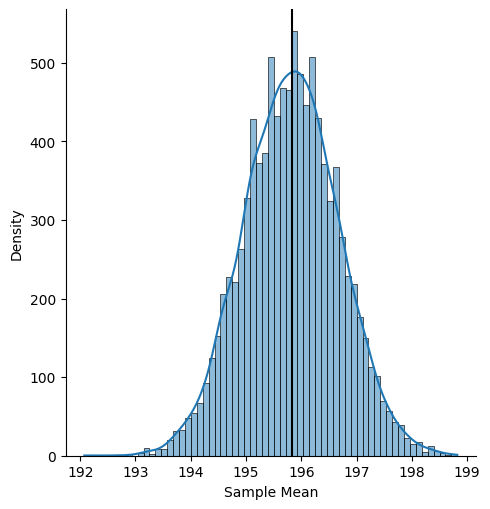
We can then compute the confidence interval with the quantiles of this distribution:
np.quantile(boot_means, [0.025, 0.975])
array([194.14705882, 197.5 ])
Penguin Statistics#
With that warmup, let’s look at our various biometrics.
Parametric Estimates#
We’re going to compute CIs for several measurements, but we don’t want to repeat all of our code.
Pandas groupby let us apply a function to each group, which can in turn return a series or a data frame.
Let’s write a function that, given a series of penguin data, returns our statistics:
def mean_estimate(vals):
    # vals is a series of measurements of a single variable
    mean = vals.mean()
    se = vals.sem()  # Pandas has an SEM function too.

    ci_width = 1.96 * se
    return pd.Series({
        'mean': mean,
        'std': vals.std(),
        'count': vals.count(),
        'se': vals.sem(),
        'ci_width': ci_width,
        'ci_min': mean - ci_width,
        'ci_max': mean + ci_width
    })
Flipper Length#
Now we can do this to the flipper length:
penguins.groupby('species')['FlipperLength'].apply(mean_estimate).unstack()
| mean | std | count | se | ci_width | ci_min | ci_max | |
|---|---|---|---|---|---|---|---|
| species | |||||||
| Adelie | 189.953642 | 6.539457 | 151.0 | 0.532173 | 1.043060 | 188.910582 | 190.996702 |
| Chinstrap | 195.823529 | 7.131894 | 68.0 | 0.864869 | 1.695144 | 194.128386 | 197.518673 |
| Gentoo | 217.186992 | 6.484976 | 123.0 | 0.584731 | 1.146072 | 216.040920 | 218.333064 |
The confidence intervals don’t overlap. Chinstrap and Adelie are the closest.
Note
The unstack function pivots the innermost level of a hierarchical index to be column labels. Try without it to see what changes!
Bill Length#
penguins.groupby('species')['BillLength'].apply(mean_estimate).unstack()
| mean | std | count | se | ci_width | ci_min | ci_max | |
|---|---|---|---|---|---|---|---|
| species | |||||||
| Adelie | 38.791391 | 2.663405 | 151.0 | 0.216745 | 0.424820 | 38.366571 | 39.216211 |
| Chinstrap | 48.833824 | 3.339256 | 68.0 | 0.404944 | 0.793691 | 48.040133 | 49.627514 |
| Gentoo | 47.504878 | 3.081857 | 123.0 | 0.277882 | 0.544648 | 46.960230 | 48.049526 |
Chinstrap and Gentoo have similar average bill depths - those CIs are very close.
Bill Depth#
penguins.groupby('species')['BillDepth'].apply(mean_estimate).unstack()
| mean | std | count | se | ci_width | ci_min | ci_max | |
|---|---|---|---|---|---|---|---|
| species | |||||||
| Adelie | 18.346358 | 1.216650 | 151.0 | 0.099010 | 0.194059 | 18.152299 | 18.540416 |
| Chinstrap | 18.420588 | 1.135395 | 68.0 | 0.137687 | 0.269866 | 18.150722 | 18.690455 |
| Gentoo | 14.982114 | 0.981220 | 123.0 | 0.088474 | 0.173408 | 14.808706 | 15.155522 |
The bill depth between Chinstrap and Adelie is extremely similar. Gentoo penguins look like they have smaller bills.
Mass#
Finally, let’s look at body mass.
penguins.groupby('species')['Mass'].apply(mean_estimate).unstack()
| mean | std | count | se | ci_width | ci_min | ci_max | |
|---|---|---|---|---|---|---|---|
| species | |||||||
| Adelie | 3700.662252 | 458.566126 | 151.0 | 37.317582 | 73.142461 | 3627.519791 | 3773.804713 |
| Chinstrap | 3733.088235 | 384.335081 | 68.0 | 46.607475 | 91.350650 | 3641.737585 | 3824.438885 |
| Gentoo | 5076.016260 | 504.116237 | 123.0 | 45.454630 | 89.091075 | 4986.925185 | 5165.107336 |
Adelie and Chinstrap are very similar, with Gentoo substantially larger. Look at the CI intervals again!
Bootstrap#
Now we’re going to bootstrap confidence intervals. I’m just going to do it for the flipper length — you should try it for the others!
Let’s take that bootstrap logic from beofre and put it in a function:
def boot_mean_estimate(vals, nboot=10000):
    obs = vals.dropna()  # ignore missing values
    mean = obs.mean()
    n = obs.count()

    boot_means = [np.mean(rng.choice(obs, size=n)) for i in range(nboot)]
    ci_low, ci_high = np.quantile(boot_means, [0.025, 0.975])
    return pd.Series({
        'mean': mean,
        'count': n,
        'ci_low': ci_low,
        'ci_high': ci_high
    })
penguins.groupby('species')['FlipperLength'].apply(boot_mean_estimate).unstack()
| mean | count | ci_low | ci_high | |
|---|---|---|---|---|
| species | ||||
| Adelie | 189.953642 | 151.0 | 188.907285 | 190.980132 |
| Chinstrap | 195.823529 | 68.0 | 194.161765 | 197.500000 |
| Gentoo | 217.186992 | 123.0 | 216.032520 | 218.357724 |
Tip
The apply function also allows us to pass additional named parameters, which are passed directly to the function we are invoking.
penguins.groupby('species')['FlipperLength'].apply(boot_mean_estimate, nboot=5000).unstack()
| mean | count | ci_low | ci_high | |
|---|---|---|---|---|
| species | ||||
| Adelie | 189.953642 | 151.0 | 188.874172 | 191.033113 |
| Chinstrap | 195.823529 | 68.0 | 194.147059 | 197.500000 |
| Gentoo | 217.186992 | 123.0 | 216.048780 | 218.341463 |
This is the interval Seaborn uses in a catplot of the statistic:
sns.catplot(x='species', y='FlipperLength', data=penguins, kind='bar')
<seaborn.axisgrid.FacetGrid at 0x238b4196f50>
Testing#
Let’s do a t-test for whether the chinstrap and adelie have different flipper lengths. The ttest_ind function does a two-sample T-test:
sps.ttest_ind(adelies['FlipperLength'], chinstraps['FlipperLength'], nan_policy='omit', equal_var=False)
Ttest_indResult(statistic=-5.780384584564813, pvalue=6.049266635901914e-08)
\(p < 0.05\), that’s for sure! The probability of observing mean flipper lengths this different if there is no actual difference is quite low.
Let’s try the bill depth:
sps.ttest_ind(adelies['BillDepth'], chinstraps['BillDepth'], nan_policy='omit')
Ttest_indResult(statistic=-0.4263555696052568, pvalue=0.6702714045724318)
\(p>0.05\). Very. The evidence is not sufficient to reject the null hypothesis that Adelie and Chinstrap penguins have the same bill depth.
Bootstrapped Test#
What about the bootstrap? Remember that to do the bootstrap, we need to resample from the pool of measurements, because the procedure is to take bootstrap samples from the distribution under the null hypothesis, which is that there is no difference between penguins.
We’ll work through it a piece at a time, then define a function.
First, we need to drop the null values from our observations:
obs1 = adelies['FlipperLength'].dropna()
obs2 = chinstraps['FlipperLength'].dropna()
And the lengths:
n1 = len(obs1)
n2 = len(obs2)
And the observed difference in means (since the mean is the statistic we are bootstrapping):
diff_mean = np.mean(obs1) - np.mean(obs2)
diff_mean
-5.869887027658734
Now we’re going to pool together the observations, so we can simulate the null hypothesis (data drawn from the same distribution):
pool = pd.concat([obs1, obs2])
pool
0      181.0
1      186.0
2      195.0
4      193.0
5      190.0
       ...
339    207.0
340    202.0
341    193.0
342    210.0
343    198.0
Name: FlipperLength, Length: 219, dtype: float64
With the pool, we can now sample bootstrap samples of the means of samples of size \(n_1\) and \(n_2\) from a merged pool:
b1 = np.array([np.mean(rng.choice(pool, size=n1)) for i in range(10000)])
b2 = np.array([np.mean(rng.choice(pool, size=n2)) for i in range(10000)])
We use the list comprehension from before, but this time we wrap its result in np.array to make NumPy arrays that support vectorized computation (lists do not). That then allows us to compute the difference in means for all bootstrap samples in one go:
boot_diffs = b1 - b2
boot_diffs
array([-0.88206077, -0.28632645, -0.25350604, ...,  0.93523568,
       -0.85196728, -0.31077133])
Now, our goal is to compute \(p\), the probability of observing a difference at least as large as diff_mean (in absolute value) under the null hypothesis \(H_0\) (the samples are from the same distribution). So we want to compute the absolute values of the differences, both bootstrapped and observed. NumPy helpfully vectorizes this:
abs_diff_mean = np.abs(diff_mean)
abs_diff_mean
5.869887027658734
abs_boot_diffs = np.abs(boot_diffs)
abs_boot_diffs
array([0.88206077, 0.28632645, 0.25350604, ..., 0.93523568, 0.85196728,
       0.31077133])
And now we can actually compare. The >= operator compares the bootstrapped differences with observed, giving us a logical vector that is True when a bootstrapped difference is at least as large as the observed difference:
boot_exceeds_observed = abs_boot_diffs >= abs_diff_mean
boot_exceeds_observed
array([False, False, False, ..., False, False, False])
Finally, we want to covert this to an estimated \(p\)-value. The np.mean function, when applied to a boolean array, returns the fraction of elements that are True:
np.mean(boot_exceeds_observed)
0.0
No elements were True (if we ran with a much larger bootstrap sample count, we might see a small number of True values). Since our bootstrap sample count estimates the \(p\)-value to approximately 5 decimal places, we conclude that the difference is statistically significant.
Bootstrap Test Function#
Let’s go! We’re going to put all that logic into a short function for easy reuse. Note that variables assigned within a function are local variables: they only have their values within the function, without affecting the global variables of the same name.
def boot_ind(s1, s2, nboot=10000):
    ## we will ignore NAs here
    obs1 = s1.dropna()
    obs2 = s2.dropna()
    n1 = len(obs1)
    n2 = len(obs2)

    ## pool the observations together
    pool = pd.concat([obs1, obs2])
    ## grab the observed mean
    md = np.mean(s1) - np.mean(s2)

    ## compute our bootstrap samples of the mean under H0
    b1 = np.array([np.mean(rng.choice(pool, size=n1)) for i in range(nboot)])
    b2 = np.array([np.mean(rng.choice(pool, size=n2)) for i in range(nboot)])

    ## the P-value is the probability that we observe a difference as large
    ## as we did in the raw data, if the null hypothesis were true
    return md, np.mean(np.abs(b1 - b2) >= np.abs(md))
And with this function, we can compute the bootstrap versions of the tests above:
boot_ind(adelies['FlipperLength'], chinstraps['FlipperLength'])
(-5.869887027658734, 0.0)
The \(p\)-value was very small in the \(t\)-test; it makes sense that we would almost never actually see a mean this large under the null!
Let’s do the bill depth:
boot_ind(adelies['BillDepth'], chinstraps['BillDepth'])
(-0.07423061940007614, 0.6724)
Yeah, those kinds of penguins seem to have the same bill depth.
Conclusion#
We see extremely similar \(p\)-values and confidence intervals for the parameteric methods and the bootstrap. That is expected — if two procedures that claimed to do the same thing returned wildly different results, we would have a problem.
But as we discussed in the videos, the bootstrap works in places where the parametrics won’t.