Sampling Distributions

This notebook has the plots and code to support the sampling, confidence, and boostrap lecture.

Setup

Python modules:

import numpy as np
import pandas as pd
import scipy.stats as sps
import matplotlib.pyplot as plt
import seaborn as sns

Set up a random number generator:

rng = np.random.default_rng(20200912)

Load the Penguin data:

penguins = pd.read_csv('../penguins.csv')

And we’re going to want to look at just the chinstraps sometimes:

chinstraps = penguins[penguins['species'] == 'Chinstrap']
chinstraps.head()

	species	island	bill_length_mm	bill_depth_mm	flipper_length_mm	body_mass_g	sex	year
276	Chinstrap	Dream	46.5	17.9	192.0	3500.0	female	2007
277	Chinstrap	Dream	50.0	19.5	196.0	3900.0	male	2007
278	Chinstrap	Dream	51.3	19.2	193.0	3650.0	male	2007
279	Chinstrap	Dream	45.4	18.7	188.0	3525.0	female	2007
280	Chinstrap	Dream	52.7	19.8	197.0	3725.0	male	2007

That’s all we need this time!

Sampling Distributions

Let’s say we have a population that is accurately described by the normal distribution \(\mathrm{Normal(50, 5)}\) — the population mean \(\mu = 50\) and its standard deviation \(\sigma = 5\), and it’s normal.

We can draw a sample of size 50 from this distribution:

dist = sps.norm(50, 5)

sample = dist.rvs(size=50, random_state=rng)

And show its distribution:

sns.displot(sample, kde=True)

<seaborn.axisgrid.FacetGrid at 0x1ded8c58610>

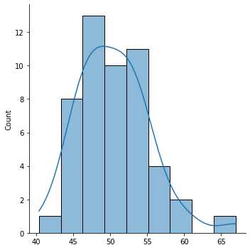
Note: The curve in a Seaborn distplot is the kernel density estimate: it is an estimate of the probability density function.

We can also compute statistics, such as the mean:

np.mean(sample)

50.462609949153304

That mean is pretty close to our true population mean of 50! But it isn’t quite exact - any given sample is going to have some error. There is natural variation in samples that affects the statistic.

But what if we did this 1000 times? And each time, we took another sample of 100, and computed its mean?

How would this sample of sample means be distributed?

Note: The syntax [expr for var in iterable] is a list comprehension. It lets is quickly write lists based on loops.

sample_means = [np.mean(dist.rvs(size=50, random_state=rng)) for i in range(1000)]
sns.displot(sample_means, kde=True)

<seaborn.axisgrid.FacetGrid at 0x1ded8cdb220>

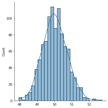
We call this distribution the sampling distribution of a statistic.

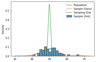
Let’s overlay these on top of each other:

plt.plot(np.linspace(30, 70), dist.pdf(np.linspace(30, 70)), label='Population')
sns.histplot(sample, label='Sample (Hist)', stat='density', bins=20)
sns.kdeplot(sample, label='Sample (Dens)')
sns.kdeplot(sample_means, label='Sampling Dist')
plt.legend()
plt.show()

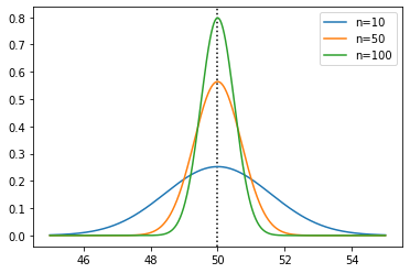
The sample mean is normally distributed with mean \(\mu\) and standard deviation \(\sigma/\sqrt{n}\). Let’s see that for a few sample sizes, with the true mean plotted as a vertical line:

xs = np.linspace(45, 55, 1000)
plt.axvline(50, color='black', linestyle=':')
plt.plot(xs, sps.norm(50, 5 / np.sqrt(10)).pdf(xs), label='n=10')
plt.plot(xs, sps.norm(50, 5 / np.sqrt(50)).pdf(xs), label='n=50')
plt.plot(xs, sps.norm(50, 5 / np.sqrt(100)).pdf(xs), label='n=100')
plt.legend()
plt.show()

Confidence Intervals

I’m going to write a little function for computing confidence intervals. It will return a (low, high) tuple.

def ci95(mean, sd, n, width=1.96):
    se = sd / np.sqrt(n)
    off = se * width
    return mean - off, mean + off

What’s the estimated CI from our sample?

Note: ddof=1 tells NumPy’s std function to compute the sample standard deviation.

ci95(np.mean(sample), np.std(sample, ddof=1), 50)

(49.113141238970556, 51.81207865933605)

Remember from the video and Confidence in Confidence.

What’s the range of the middle 95% if we do it a thousand times? Since we can, of course!

def samp_ci(size=50):
    sample = dist.rvs(size=size, random_state=rng)
    mean = np.mean(sample)
    std = np.std(sample, ddof=1)
    return ci95(mean, std, size)

We’re going to use this function with another trick for building Pandas data frames — the from_records function, to build from an iterable of rows. This will give us 1000 intervals:

samp_cis = pd.DataFrame.from_records(
    [samp_ci() for i in range(1000)],
    columns=['lo', 'hi']
)
samp_cis

	lo	hi
0	48.460558	51.501088
1	49.713563	53.065665
2	47.943036	50.575633
3	48.858734	51.382044
4	48.087636	50.666545
...	...	...
995	48.148537	50.703322
996	48.171565	50.644276
997	48.252690	50.419871
998	48.022458	50.543743
999	48.544989	51.381232

1000 rows × 2 columns

Mark the samples where it contains the true mean of 50, and see what fraction there are:

samp_cis['hit'] = (samp_cis['lo'] <= 50) & (samp_cis['hi'] >= 50)
samp_cis.mean()

lo     48.604607
hi     51.358654
hit     0.940000
dtype: float64

94% of our confindence intervals contain the mean. That is quite close to 95%.

Practice: we can treat ‘confidence interval contains the true mean’ as an event with 95% probability of success. What distribution describes the number of expected successess for 1000 trials at 95% success? What is the probability that we would see a value in the range \(950 \pm 10\) for such a set of trials?