Correlation and Basic Linear Model
Contents
Correlation and Basic Linear Model#
This notebook shows how to draw scatter plots, compute correlations, and fit a basic linear model.
It accompanies Week 6 and Week 8.
Setup and Data#
Let’s load our Python modules. We’re adding two new ones:
statsmodels.api— the core Statsmodels APIsstatsmodels.formula.api— convenience APIs for Statsmodels that let us specify models with formulae
import pandas as pd
import numpy as np
import statsmodels.api as sm
import statsmodels.formula.api as smf
import matplotlib.pyplot as plt
import seaborn as sns
And load our data - this is the HetRec data we’ve been using a lot:
movies = pd.read_csv('hetrec2011-ml/movies.dat', encoding='latin1', delimiter='\t', na_values='\\N')
movies
| id | title | imdbID | spanishTitle | imdbPictureURL | year | rtID | rtAllCriticsRating | rtAllCriticsNumReviews | rtAllCriticsNumFresh | ... | rtAllCriticsScore | rtTopCriticsRating | rtTopCriticsNumReviews | rtTopCriticsNumFresh | rtTopCriticsNumRotten | rtTopCriticsScore | rtAudienceRating | rtAudienceNumRatings | rtAudienceScore | rtPictureURL | |
|---|---|---|---|---|---|---|---|---|---|---|---|---|---|---|---|---|---|---|---|---|---|
| 0 | 1 | Toy story | 114709 | Toy story (juguetes) | http://ia.media-imdb.com/images/M/MV5BMTMwNDU0... | 1995 | toy_story | 9.0 | 73.0 | 73.0 | ... | 100.0 | 8.5 | 17.0 | 17.0 | 0.0 | 100.0 | 3.7 | 102338.0 | 81.0 | http://content7.flixster.com/movie/10/93/63/10... |
| 1 | 2 | Jumanji | 113497 | Jumanji | http://ia.media-imdb.com/images/M/MV5BMzM5NjE1... | 1995 | 1068044-jumanji | 5.6 | 28.0 | 13.0 | ... | 46.0 | 5.8 | 5.0 | 2.0 | 3.0 | 40.0 | 3.2 | 44587.0 | 61.0 | http://content8.flixster.com/movie/56/79/73/56... |
| 2 | 3 | Grumpy Old Men | 107050 | Dos viejos gruñones | http://ia.media-imdb.com/images/M/MV5BMTI5MTgy... | 1993 | grumpy_old_men | 5.9 | 36.0 | 24.0 | ... | 66.0 | 7.0 | 6.0 | 5.0 | 1.0 | 83.0 | 3.2 | 10489.0 | 66.0 | http://content6.flixster.com/movie/25/60/25602... |
| 3 | 4 | Waiting to Exhale | 114885 | Esperando un respiro | http://ia.media-imdb.com/images/M/MV5BMTczMTMy... | 1995 | waiting_to_exhale | 5.6 | 25.0 | 14.0 | ... | 56.0 | 5.5 | 11.0 | 5.0 | 6.0 | 45.0 | 3.3 | 5666.0 | 79.0 | http://content9.flixster.com/movie/10/94/17/10... |
| 4 | 5 | Father of the Bride Part II | 113041 | Vuelve el padre de la novia (Ahora también abu... | http://ia.media-imdb.com/images/M/MV5BMTg1NDc2... | 1995 | father_of_the_bride_part_ii | 5.3 | 19.0 | 9.0 | ... | 47.0 | 5.4 | 5.0 | 1.0 | 4.0 | 20.0 | 3.0 | 13761.0 | 64.0 | http://content8.flixster.com/movie/25/54/25542... |
| ... | ... | ... | ... | ... | ... | ... | ... | ... | ... | ... | ... | ... | ... | ... | ... | ... | ... | ... | ... | ... | ... |
| 10192 | 65088 | Bedtime Stories | 960731 | Más allá de los sueños | http://ia.media-imdb.com/images/M/MV5BMjA5Njk5... | 2008 | bedtime_stories | 4.4 | 104.0 | 26.0 | ... | 25.0 | 4.7 | 26.0 | 6.0 | 20.0 | 23.0 | 3.5 | 108877.0 | 63.0 | http://content6.flixster.com/movie/10/94/33/10... |
| 10193 | 65091 | Manhattan Melodrama | 25464 | El enemigo público número 1 | http://ia.media-imdb.com/images/M/MV5BMTUyODE3... | 1934 | manhattan_melodrama | 7.0 | 12.0 | 10.0 | ... | 83.0 | 0.0 | 4.0 | 2.0 | 2.0 | 50.0 | 3.7 | 344.0 | 71.0 | http://content9.flixster.com/movie/66/44/64/66... |
| 10194 | 65126 | Choke | 1024715 | Choke | http://ia.media-imdb.com/images/M/MV5BMTMxMDI4... | 2008 | choke | 5.6 | 135.0 | 73.0 | ... | 54.0 | 4.9 | 26.0 | 8.0 | 18.0 | 30.0 | 3.3 | 13893.0 | 55.0 | http://content6.flixster.com/movie/10/85/09/10... |
| 10195 | 65130 | Revolutionary Road | 959337 | Revolutionary Road | http://ia.media-imdb.com/images/M/MV5BMTI2MzY2... | 2008 | revolutionary_road | 6.7 | 194.0 | 133.0 | ... | 68.0 | 6.9 | 36.0 | 25.0 | 11.0 | 69.0 | 3.5 | 46044.0 | 70.0 | http://content8.flixster.com/movie/10/88/40/10... |
| 10196 | 65133 | Blackadder Back & Forth | 212579 | Blackadder Back & Forth | http://ia.media-imdb.com/images/M/MV5BMjA5MjU4... | 1999 | blackadder-back-forth | 0.0 | 0.0 | 0.0 | ... | 0.0 | 0.0 | 0.0 | 0.0 | 0.0 | 0.0 | 0.0 | 0.0 | 0.0 | http://content7.flixster.com/movie/34/10/69/34... |
10197 rows × 21 columns
movies.info()
<class 'pandas.core.frame.DataFrame'>
RangeIndex: 10197 entries, 0 to 10196
Data columns (total 21 columns):
 #   Column                  Non-Null Count  Dtype
---  ------                  --------------  -----
 0   id                      10197 non-null  int64
 1   title                   10197 non-null  object
 2   imdbID                  10197 non-null  int64
 3   spanishTitle            10197 non-null  object
 4   imdbPictureURL          10016 non-null  object
 5   year                    10197 non-null  int64
 6   rtID                    9886 non-null   object
 7   rtAllCriticsRating      9967 non-null   float64
 8   rtAllCriticsNumReviews  9967 non-null   float64
 9   rtAllCriticsNumFresh    9967 non-null   float64
 10  rtAllCriticsNumRotten   9967 non-null   float64
 11  rtAllCriticsScore       9967 non-null   float64
 12  rtTopCriticsRating      9967 non-null   float64
 13  rtTopCriticsNumReviews  9967 non-null   float64
 14  rtTopCriticsNumFresh    9967 non-null   float64
 15  rtTopCriticsNumRotten   9967 non-null   float64
 16  rtTopCriticsScore       9967 non-null   float64
 17  rtAudienceRating        9967 non-null   float64
 18  rtAudienceNumRatings    9967 non-null   float64
 19  rtAudienceScore         9967 non-null   float64
 20  rtPictureURL            9967 non-null   object
dtypes: float64(13), int64(3), object(5)
memory usage: 1.6+ MB
Following Missing Data, we’re going to clear out the critic & audience ratings that are clearly incorrectly-coded missing data:
movies.loc[movies['rtAllCriticsRating'] == 0, 'rtAllCriticsRating'] = np.nan
movies.loc[movies['rtTopCriticsRating'] == 0, 'rtTopCriticsRating'] = np.nan
movies.loc[movies['rtAudienceRating'] == 0, 'rtAudienceRating'] = np.nan
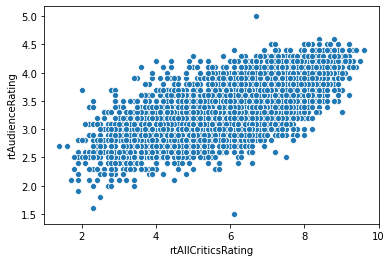
Scatterplots#
Our fundamental way to show two numeric variable is a scatterplot:
sns.scatterplot('rtAllCriticsRating', 'rtAudienceRating', data=movies)
plt.show()
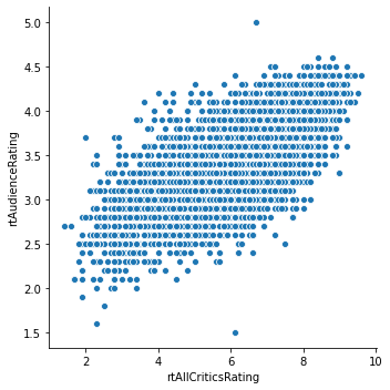
The relplot does the same thing, but is a Seaborn figure-level plot (meaning it controls the entire matplotlib drawing process, including figure size):
sns.relplot('rtAllCriticsRating', 'rtAudienceRating', data=movies)
plt.show()
Joint Plot#
If we also want to show the marginal distributions (the distributions of individual variables), we can use a jointplot:
sns.jointplot('rtAllCriticsRating', 'rtAudienceRating', data=movies)
plt.show()
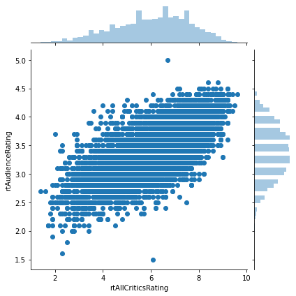
These plots are exceptionally useful in exporatory analysis.
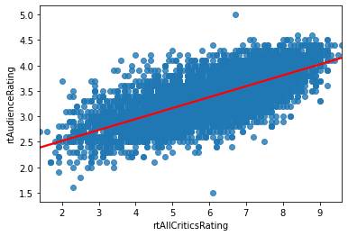
Trend Line#
And we can draw a scatterplot with a trend line using regplot (here I am specifying additional line options, line_kws, to make the line visibile as a different color):
sns.regplot('rtAllCriticsRating', 'rtAudienceRating', data=movies, line_kws={'color': 'red'})
<matplotlib.axes._subplots.AxesSubplot at 0x20f967224c0>
Scatterplot Matrix#
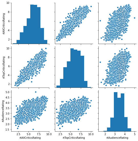
If we want to view relationships between more than 2 variables, we can look at the individual pairwise potential relationships through a scatterplot matrix (Seaborn pairplot):
sns.pairplot(movies[['rtAllCriticsRating', 'rtTopCriticsRating', 'rtAudienceRating']])
<seaborn.axisgrid.PairGrid at 0x20f9684f1c0>
Correlation and Covariance#
The Pandas cov method computes covariance between two series:
movies['rtAllCriticsRating'].cov(movies['rtTopCriticsRating'])
2.1505561772886375
Covariance is symmetric:
movies['rtTopCriticsRating'].cov(movies['rtAllCriticsRating'])
2.1505561772886375
By default, it also ignores observations with missing values.
The pandas.Series.corr() method computes the correlation coefficient \(-1 \le r \le 1\), that is independent of the variance or scale of the data (1 always means perfect correlation):
movies['rtAllCriticsRating'].corr(movies['rtTopCriticsRating'])
0.934600465561324
That is a high correlation for almost any purpose.
We can also compute a correlation matrix by calling .corr on a data frame:
movies[['rtAllCriticsRating', 'rtTopCriticsRating', 'rtAudienceRating']].corr()
| rtAllCriticsRating | rtTopCriticsRating | rtAudienceRating | |
|---|---|---|---|
| rtAllCriticsRating | 1.000000 | 0.934600 | 0.718364 |
| rtTopCriticsRating | 0.934600 | 1.000000 | 0.627785 |
| rtAudienceRating | 0.718364 | 0.627785 | 1.000000 |
This shows the correlation between each pair of variables. The correlation of a variable with itself is always 1 (and the covariance of a variable with itself is its variance — do the algebra to convince yourself why!). Audience and top critics are not as well-correlated as the two critic sources, or audience with all critics.
Bootstrapping the Correlation#
We can use the bootstrap to compute a confidence interval for the correlation between two variables. Let’s do that for audience and top-critics ratings.
We’ll start by making a frame that just has those columns, with NAs removed:
crit_movies = movies.set_index('id')[['rtTopCriticsRating', 'rtAudienceRating']].dropna()
And compute the correlation, for reference:
crit_movies['rtTopCriticsRating'].corr(crit_movies['rtAudienceRating'])
0.6277851818091278
Now let’s bootstrap that. We’ll bootstrap 10000 times. This time we will use a for loop, just to demonstrate that. We’re also going to use the Pandas sample method, to sample rows of a data frame (and thus pairs of observations). To bootstrap a correlation, we can’t just sample individual values!
NBOOT = 10000
boot_corrs = np.empty(NBOOT)
for i in range(NBOOT):
samp = crit_movies.sample(n=len(crit_movies), replace=True)
boot_corrs[i] = samp['rtTopCriticsRating'].corr(samp['rtAudienceRating'])
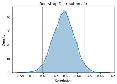
np.quantile(boot_corrs, [0.025, 0.975])
array([0.60939528, 0.64571617])
We can also see the approximated sampling distribution:
sns.distplot(boot_corrs)
lb, ub = np.quantile(boot_corrs, [0.025, 0.975])
plt.axvline(lb, color='grey')
plt.axvline(ub, color='grey')
plt.title('Bootstrap Distribution of r')
plt.ylabel('Density')
plt.xlabel('Correlation')
plt.show()
Regression#
Finally, I want to show you how to fit the regression model:
mod = smf.ols('rtAudienceRating ~ rtTopCriticsRating', data=movies)
res = mod.fit()
res.summary()
| Dep. Variable: | rtAudienceRating | R-squared: | 0.394 |
|---|---|---|---|
| Model: | OLS | Adj. R-squared: | 0.394 |
| Method: | Least Squares | F-statistic: | 3012. |
| Date: | Sat, 10 Oct 2020 | Prob (F-statistic): | 0.00 |
| Time: | 12:28:47 | Log-Likelihood: | -1701.8 |
| No. Observations: | 4632 | AIC: | 3408. |
| Df Residuals: | 4630 | BIC: | 3421. |
| Df Model: | 1 | ||
| Covariance Type: | nonrobust |
| coef | std err | t | P>|t| | [0.025 | 0.975] | |
|---|---|---|---|---|---|---|
| Intercept | 2.2847 | 0.021 | 111.441 | 0.000 | 2.245 | 2.325 |
| rtTopCriticsRating | 0.1838 | 0.003 | 54.879 | 0.000 | 0.177 | 0.190 |
| Omnibus: | 3.451 | Durbin-Watson: | 1.825 |
|---|---|---|---|
| Prob(Omnibus): | 0.178 | Jarque-Bera (JB): | 3.414 |
| Skew: | -0.053 | Prob(JB): | 0.181 |
| Kurtosis: | 3.079 | Cond. No. | 25.1 |
Warnings:
[1] Standard Errors assume that the covariance matrix of the errors is correctly specified.
For now, we need to ignore the p-value.
Fitting this model has resulted in “learining” the following line, where \(y\) is the audience rating and \(x\) the critic rating:
This means that we have used the data to “learn” the parameters (coefficient and intercept) for a linear model to predict the data. That’s all (supervised) machine learning is!
Later we’re going to see why, but we want check the residuals for normality:
sm.qqplot(res.resid, fit=True, line='45')
plt.show()
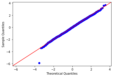
Looks good! One outlier.
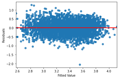
Let’s also look at the residuals vs. fitted plot, to test for equal variance:
sns.regplot(res.fittedvalues, res.resid, line_kws={'color': 'red'})
plt.xlabel('Fitted Value')
plt.ylabel('Residuals')
plt.show()
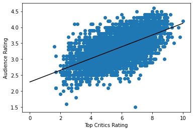
I’m also going to plot the regression line ourselves:
plt.scatter(movies['rtTopCriticsRating'], movies['rtAudienceRating'])
l_xs = np.linspace(0, 10, 100)
l_ys = res.params[0] + res.params[1] * l_xs
plt.plot(l_xs, l_ys, color='black')
plt.xlabel('Top Critics Rating')
plt.ylabel('Audience Rating')
plt.show()
Predictive Accuracy#
Now, we should have done this before we started fitting any models. We will adopt proper splitting in the future.
We’re going to make train and test sets:
predictable = movies.dropna(subset=['rtTopCriticsRating', 'rtAudienceRating'])
predictable.info()
<class 'pandas.core.frame.DataFrame'>
Int64Index: 4632 entries, 0 to 10195
Data columns (total 21 columns):
 #   Column                  Non-Null Count  Dtype
---  ------                  --------------  -----
 0   id                      4632 non-null   int64
 1   title                   4632 non-null   object
 2   imdbID                  4632 non-null   int64
 3   spanishTitle            4632 non-null   object
 4   imdbPictureURL          4603 non-null   object
 5   year                    4632 non-null   int64
 6   rtID                    4603 non-null   object
 7   rtAllCriticsRating      4632 non-null   float64
 8   rtAllCriticsNumReviews  4632 non-null   float64
 9   rtAllCriticsNumFresh    4632 non-null   float64
 10  rtAllCriticsNumRotten   4632 non-null   float64
 11  rtAllCriticsScore       4632 non-null   float64
 12  rtTopCriticsRating      4632 non-null   float64
 13  rtTopCriticsNumReviews  4632 non-null   float64
 14  rtTopCriticsNumFresh    4632 non-null   float64
 15  rtTopCriticsNumRotten   4632 non-null   float64
 16  rtTopCriticsScore       4632 non-null   float64
 17  rtAudienceRating        4632 non-null   float64
 18  rtAudienceNumRatings    4632 non-null   float64
 19  rtAudienceScore         4632 non-null   float64
 20  rtPictureURL            4632 non-null   object
dtypes: float64(13), int64(3), object(5)
memory usage: 796.1+ KB
Sample 20% of movies as test data:
test = predictable.sample(frac=0.2)
Create a mask and use it to pick the rest as training data:
train_mask = pd.Series(True, index=predictable.index)
train_mask[test.index] = False
train = predictable[train_mask]
Fit the model:
pmod = smf.ols('rtAudienceRating ~ rtTopCriticsRating', data=train)
pfit = pmod.fit()
pfit.summary()
| Dep. Variable: | rtAudienceRating | R-squared: | 0.389 |
|---|---|---|---|
| Model: | OLS | Adj. R-squared: | 0.389 |
| Method: | Least Squares | F-statistic: | 2359. |
| Date: | Sat, 10 Oct 2020 | Prob (F-statistic): | 0.00 |
| Time: | 12:28:48 | Log-Likelihood: | -1400.3 |
| No. Observations: | 3706 | AIC: | 2805. |
| Df Residuals: | 3704 | BIC: | 2817. |
| Df Model: | 1 | ||
| Covariance Type: | nonrobust |
| coef | std err | t | P>|t| | [0.025 | 0.975] | |
|---|---|---|---|---|---|---|
| Intercept | 2.2852 | 0.023 | 98.873 | 0.000 | 2.240 | 2.331 |
| rtTopCriticsRating | 0.1832 | 0.004 | 48.567 | 0.000 | 0.176 | 0.191 |
| Omnibus: | 2.666 | Durbin-Watson: | 1.837 |
|---|---|---|---|
| Prob(Omnibus): | 0.264 | Jarque-Bera (JB): | 2.606 |
| Skew: | -0.062 | Prob(JB): | 0.272 |
| Kurtosis: | 3.042 | Cond. No. | 25.0 |
Warnings:
[1] Standard Errors assume that the covariance matrix of the errors is correctly specified.
preds = pfit.predict(test)
test['predAud'] = preds
test
| id | title | imdbID | spanishTitle | imdbPictureURL | year | rtID | rtAllCriticsRating | rtAllCriticsNumReviews | rtAllCriticsNumFresh | ... | rtTopCriticsRating | rtTopCriticsNumReviews | rtTopCriticsNumFresh | rtTopCriticsNumRotten | rtTopCriticsScore | rtAudienceRating | rtAudienceNumRatings | rtAudienceScore | rtPictureURL | predAud | |
|---|---|---|---|---|---|---|---|---|---|---|---|---|---|---|---|---|---|---|---|---|---|
| 9775 | 58029 | It's a Free World... | 807054 | En un mundo libre... | http://ia.media-imdb.com/images/M/MV5BMjEzMjY3... | 2007 | its_a_free_world | 6.6 | 18.0 | 15.0 | ... | 6.2 | 6.0 | 4.0 | 2.0 | 66.0 | 3.6 | 1788.0 | 70.0 | http://content7.flixster.com/movie/10/49/04/10... | 3.421068 |
| 8367 | 27741 | Tasogare Seibei | 351817 | El ocaso del samurái | http://ia.media-imdb.com/images/M/MV5BMTgzMTA1... | 2002 | twilight_samurai | 8.2 | 68.0 | 67.0 | ... | 7.9 | 22.0 | 22.0 | 0.0 | 100.0 | 4.2 | 3512.0 | 93.0 | http://content9.flixster.com/movie/10/92/29/10... | 3.732509 |
| 9343 | 49644 | Off the Black | 479965 | Off the Black | http://ia.media-imdb.com/images/M/MV5BMTc1NzIw... | 2006 | off_the_black | 6.2 | 40.0 | 27.0 | ... | 6.4 | 17.0 | 13.0 | 4.0 | 76.0 | 3.3 | 1007.0 | 57.0 | http://content8.flixster.com/movie/36/98/94/36... | 3.457708 |
| 8915 | 39390 | The Gospel | 451069 | The Gospel | http://ia.media-imdb.com/images/M/MV5BMTQ1Njkw... | 2005 | gospel | 4.9 | 37.0 | 12.0 | ... | 5.1 | 13.0 | 5.0 | 8.0 | 38.0 | 3.5 | 1967.0 | 78.0 | http://content8.flixster.com/movie/25/02/25029... | 3.219547 |
| 6799 | 7192 | Only the Strong | 107750 | Sólo el más fuerte | http://ia.media-imdb.com/images/M/MV5BMTY3MDQx... | 1993 | only_the_strong | 2.8 | 7.0 | 0.0 | ... | 2.5 | 5.0 | 0.0 | 5.0 | 0.0 | 3.7 | 1259.0 | 79.0 | http://content9.flixster.com/movie/10/86/99/10... | 2.743225 |
| ... | ... | ... | ... | ... | ... | ... | ... | ... | ... | ... | ... | ... | ... | ... | ... | ... | ... | ... | ... | ... | ... |
| 10050 | 62293 | The Duchess | 864761 | La duquesa | http://ia.media-imdb.com/images/M/MV5BMTU1MTQz... | 2008 | 10009493-duchess | 6.3 | 161.0 | 98.0 | ... | 6.6 | 35.0 | 24.0 | 11.0 | 68.0 | 3.5 | 22537.0 | 69.0 | http://content8.flixster.com/movie/10/85/97/10... | 3.494348 |
| 4975 | 5296 | The Sweetest Thing | 253867 | La cosa más dulce | http://ia.media-imdb.com/images/M/MV5BMTMzNDA1... | 2002 | sweetest_thing | 4.2 | 104.0 | 26.0 | ... | 4.2 | 26.0 | 7.0 | 19.0 | 26.0 | 3.0 | 21858.0 | 68.0 | http://content9.flixster.com/movie/58/56/24/58... | 3.054667 |
| 4001 | 4300 | Bread and Roses | 212826 | Pan y rosas | http://ia.media-imdb.com/images/M/MV5BMjM5MzQ2... | 2000 | bread_and_roses | 6.1 | 62.0 | 40.0 | ... | 6.3 | 21.0 | 15.0 | 6.0 | 71.0 | 3.7 | 1038.0 | 76.0 | http://content9.flixster.com/movie/74/96/53/74... | 3.439388 |
| 9043 | 43560 | Nanny McPhee | 396752 | La niñera mágica | http://ia.media-imdb.com/images/M/MV5BMTIzOTU4... | 2005 | 1153987-nanny_mcphee | 6.6 | 130.0 | 95.0 | ... | 6.4 | 29.0 | 19.0 | 10.0 | 65.0 | 3.2 | 48480.0 | 63.0 | http://content7.flixster.com/movie/10/92/77/10... | 3.457708 |
| 6595 | 6985 | La passion de Jeanne d'Arc | 19254 | La pasión de Juana de Arco | http://ia.media-imdb.com/images/M/MV5BNzExMjgz... | 1928 | passion_of_joan_of_arc | 8.9 | 31.0 | 30.0 | ... | 8.1 | 6.0 | 5.0 | 1.0 | 83.0 | 4.4 | 3362.0 | 94.0 | http://content9.flixster.com/movie/10/92/71/10... | 3.769149 |
926 rows × 22 columns
And now we’re going to compute the root mean squared error (RMSE):
test['error'] = test['rtAudienceRating'] - test['predAud']
np.sqrt(np.mean(np.square(test['error'])))
0.3343906896473175
And the mean absolute error (MAE):
np.mean(np.abs(test['error']))
0.2635027350646757