Describing Distributions
Setup
Import our modules again:
import numpy as np
import pandas as pd
import matplotlib.pyplot as plt
import seaborn as sns
And load the MovieLens data. We’re going to pass the memory_use='deep' to info, so we can see the total memory use including the strings.
movies = pd.read_csv('ml-25m/movies.csv')
movies.info(memory_usage='deep')
<class 'pandas.core.frame.DataFrame'>
RangeIndex: 62423 entries, 0 to 62422
Data columns (total 3 columns):
 #   Column   Non-Null Count  Dtype
---  ------   --------------  -----
 0   movieId  62423 non-null  int64
 1   title    62423 non-null  object
 2   genres   62423 non-null  object
dtypes: int64(1), object(2)
memory usage: 9.6 MB
ratings = pd.read_csv('ml-25m/ratings.csv')
ratings.info()
<class 'pandas.core.frame.DataFrame'>
RangeIndex: 25000095 entries, 0 to 25000094
Data columns (total 4 columns):
 #   Column     Dtype
---  ------     -----
 0   userId     int64
 1   movieId    int64
 2   rating     float64
 3   timestamp  int64
dtypes: float64(1), int64(3)
memory usage: 762.9 MB
Quickly preview the ratings frame:
ratings
| userId | movieId | rating | timestamp | |
|---|---|---|---|---|
| 0 | 1 | 296 | 5.0 | 1147880044 |
| 1 | 1 | 306 | 3.5 | 1147868817 |
| 2 | 1 | 307 | 5.0 | 1147868828 |
| 3 | 1 | 665 | 5.0 | 1147878820 |
| 4 | 1 | 899 | 3.5 | 1147868510 |
| ... | ... | ... | ... | ... |
| 25000090 | 162541 | 50872 | 4.5 | 1240953372 |
| 25000091 | 162541 | 55768 | 2.5 | 1240951998 |
| 25000092 | 162541 | 56176 | 2.0 | 1240950697 |
| 25000093 | 162541 | 58559 | 4.0 | 1240953434 |
| 25000094 | 162541 | 63876 | 5.0 | 1240952515 |
25000095 rows × 4 columns
Movie stats:
movie_stats = ratings.groupby('movieId')['rating'].agg(['mean', 'count'])
movie_stats
| mean | count | |
|---|---|---|
| movieId | ||
| 1 | 3.893708 | 57309 |
| 2 | 3.251527 | 24228 |
| 3 | 3.142028 | 11804 |
| 4 | 2.853547 | 2523 |
| 5 | 3.058434 | 11714 |
| ... | ... | ... |
| 209157 | 1.500000 | 1 |
| 209159 | 3.000000 | 1 |
| 209163 | 4.500000 | 1 |
| 209169 | 3.000000 | 1 |
| 209171 | 3.000000 | 1 |
59047 rows × 2 columns
movie_info = movies.join(movie_stats, on='movieId')
movie_info
| movieId | title | genres | mean | count | |
|---|---|---|---|---|---|
| 0 | 1 | Toy Story (1995) | Adventure|Animation|Children|Comedy|Fantasy | 3.893708 | 57309.0 |
| 1 | 2 | Jumanji (1995) | Adventure|Children|Fantasy | 3.251527 | 24228.0 |
| 2 | 3 | Grumpier Old Men (1995) | Comedy|Romance | 3.142028 | 11804.0 |
| 3 | 4 | Waiting to Exhale (1995) | Comedy|Drama|Romance | 2.853547 | 2523.0 |
| 4 | 5 | Father of the Bride Part II (1995) | Comedy | 3.058434 | 11714.0 |
| ... | ... | ... | ... | ... | ... |
| 62418 | 209157 | We (2018) | Drama | 1.500000 | 1.0 |
| 62419 | 209159 | Window of the Soul (2001) | Documentary | 3.000000 | 1.0 |
| 62420 | 209163 | Bad Poems (2018) | Comedy|Drama | 4.500000 | 1.0 |
| 62421 | 209169 | A Girl Thing (2001) | (no genres listed) | 3.000000 | 1.0 |
| 62422 | 209171 | Women of Devil's Island (1962) | Action|Adventure|Drama | 3.000000 | 1.0 |
62423 rows × 5 columns
Normal Distribution
I want to visualize an array of random, normally-distributed numbers.
We’ll first generate them:
numbers = pd.Series(np.random.randn(10000) + 5)
numbers
0       3.996778
1       4.119017
2       4.360605
3       4.850503
4       6.244754
          ...
9995    4.614897
9996    5.742292
9997    4.271137
9998    4.117684
9999    4.199830
Length: 10000, dtype: float64
And then describe them:
numbers.describe()
count    10000.000000
mean         4.998850
std          1.006624
min          1.473666
25%          4.305575
50%          4.982345
75%          5.690335
max          9.202777
dtype: float64
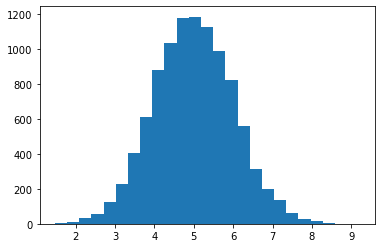
And finally visualize them:
plt.hist(numbers, bins=25)
(array([6.000e+00, 8.000e+00, 3.500e+01, 5.500e+01, 1.220e+02, 2.280e+02,
        4.070e+02, 6.110e+02, 8.810e+02, 1.033e+03, 1.175e+03, 1.184e+03,
        1.125e+03, 9.890e+02, 8.230e+02, 5.580e+02, 3.160e+02, 1.990e+02,
        1.360e+02, 6.000e+01, 2.800e+01, 1.400e+01, 6.000e+00, 0.000e+00,
        1.000e+00]),
 array([1.47366561, 1.78283007, 2.09199454, 2.401159  , 2.71032347,
        3.01948793, 3.3286524 , 3.63781687, 3.94698133, 4.2561458 ,
        4.56531026, 4.87447473, 5.18363919, 5.49280366, 5.80196812,
        6.11113259, 6.42029706, 6.72946152, 7.03862599, 7.34779045,
        7.65695492, 7.96611938, 8.27528385, 8.58444831, 8.89361278,
        9.20277725]),
 <a list of 25 Patch objects>)
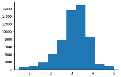
Average Movie Rating
To start looking at some real data, let’s look at the distribution of average movie rating:
movie_info['mean'].describe()
count    59047.000000
mean         3.071374
std          0.739840
min          0.500000
25%          2.687500
50%          3.150000
75%          3.500000
max          5.000000
Name: mean, dtype: float64
Let’s make a histogram:
plt.hist(movie_info['mean'])
plt.show()
C:\Users\michaelekstrand\Anaconda3\lib\site-packages\numpy\lib\histograms.py:839: RuntimeWarning: invalid value encountered in greater_equal
  keep = (tmp_a >= first_edge)
C:\Users\michaelekstrand\Anaconda3\lib\site-packages\numpy\lib\histograms.py:840: RuntimeWarning: invalid value encountered in less_equal
  keep &= (tmp_a <= last_edge)
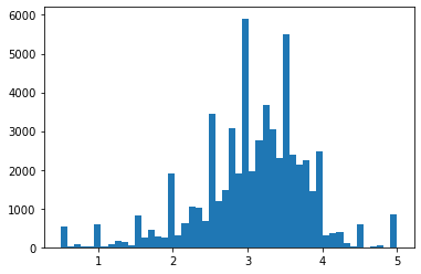
And with more bins:
plt.hist(movie_info['mean'], bins=50)
plt.show()
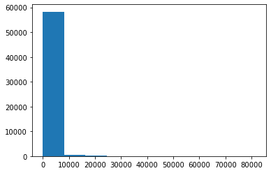
Movie Count
Now we want to describe the distribution of the ratings-per-movie (movie popularity).
movie_info['count'].describe()
count    59047.000000
mean       423.393144
std       2477.885821
min          1.000000
25%          2.000000
50%          6.000000
75%         36.000000
max      81491.000000
Name: count, dtype: float64
plt.hist(movie_info['count'])
plt.show()
plt.hist(movie_info['count'], bins=100)
plt.show()
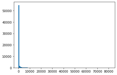
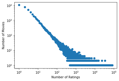
That is a very skewed distribution. Will it make more sense on a logarithmic scale?
We don’t want to just log-scale a histogram - it will be very difficult to interpret. We will use a point plot.
The value_counts() method counts the number of times each value appers. The resulting series is indexed by value, so we will use its index as the x-axis of the plot. Indexes are arrays too!
hist = movie_info['count'].value_counts()
plt.scatter(hist.index, hist)
plt.yscale('log')
plt.ylabel('Number of Movies')
plt.xscale('log')
plt.xlabel('Number of Ratings')
Text(0.5, 0, 'Number of Ratings')
Penguins
Let’s load the Penguin data (converted from R):
penguins = pd.read_csv('penguins.csv')
penguins
| species | island | bill_length_mm | bill_depth_mm | flipper_length_mm | body_mass_g | sex | year | |
|---|---|---|---|---|---|---|---|---|
| 0 | Adelie | Torgersen | 39.1 | 18.7 | 181.0 | 3750.0 | male | 2007 |
| 1 | Adelie | Torgersen | 39.5 | 17.4 | 186.0 | 3800.0 | female | 2007 |
| 2 | Adelie | Torgersen | 40.3 | 18.0 | 195.0 | 3250.0 | female | 2007 |
| 3 | Adelie | Torgersen | NaN | NaN | NaN | NaN | NaN | 2007 |
| 4 | Adelie | Torgersen | 36.7 | 19.3 | 193.0 | 3450.0 | female | 2007 |
| ... | ... | ... | ... | ... | ... | ... | ... | ... |
| 339 | Chinstrap | Dream | 55.8 | 19.8 | 207.0 | 4000.0 | male | 2009 |
| 340 | Chinstrap | Dream | 43.5 | 18.1 | 202.0 | 3400.0 | female | 2009 |
| 341 | Chinstrap | Dream | 49.6 | 18.2 | 193.0 | 3775.0 | male | 2009 |
| 342 | Chinstrap | Dream | 50.8 | 19.0 | 210.0 | 4100.0 | male | 2009 |
| 343 | Chinstrap | Dream | 50.2 | 18.7 | 198.0 | 3775.0 | female | 2009 |
344 rows × 8 columns
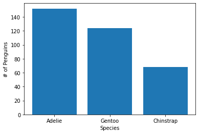
Now we’ll compute a histogram. There are ways to do this automatically, but for demonstration purposes I want to do the computations ourselves:
spec_counts = penguins['species'].value_counts()
plt.bar(spec_counts.index, spec_counts)
plt.xlabel('Species')
plt.ylabel('# of Penguins')
Text(0, 0.5, '# of Penguins')
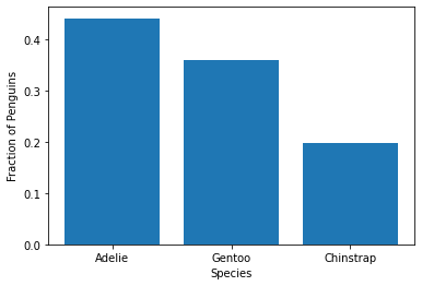
What if we want to show the fraction of each species? We can divide by the sum:
spec_fracs = spec_counts / spec_counts.sum()
plt.bar(spec_counts.index, spec_fracs)
plt.xlabel('Species')
plt.ylabel('Fraction of Penguins')
Text(0, 0.5, 'Fraction of Penguins')