Movie Matrix Decomposition¶

This notebook demonstrates matrix decomposition with the MovieLens 25M data set.

Setup¶

Import useful PyData modules:

import numpy as np
import pandas as pd
import seaborn as sns
import matplotlib.pyplot as plt
from scipy.sparse import csr_matrix

And some SciKit-Learn:

from sklearn.decomposition import TruncatedSVD

Data¶

movies = pd.read_csv('ml-25m/movies.csv')
movies.info()

<class 'pandas.core.frame.DataFrame'>
RangeIndex: 62423 entries, 0 to 62422
Data columns (total 3 columns):
 #   Column   Non-Null Count  Dtype 
---  ------   --------------  ----- 
 0   movieId  62423 non-null  int64 
 1   title    62423 non-null  object
 2   genres   62423 non-null  object
dtypes: int64(1), object(2)
memory usage: 1.4+ MB

We’re going to index that by movie ID:

movies.set_index('movieId', inplace=True)

And now load the ratings:

ratings = pd.read_csv('ml-25m/ratings.csv', dtype={
    'movieId': 'int32',
    'userId': 'int32',
    'rating': 'float32'
})
ratings.info()

<class 'pandas.core.frame.DataFrame'>
RangeIndex: 25000095 entries, 0 to 25000094
Data columns (total 4 columns):
 #   Column     Dtype  
---  ------     -----  
 0   userId     int32  
 1   movieId    int32  
 2   rating     float32
 3   timestamp  int64  
dtypes: float32(1), int32(2), int64(1)
memory usage: 476.8 MB

And load the movie tags:

tags = pd.read_csv('ml-25m/tags.csv', dtype={
    'movieId': 'int32',
    'userId': 'int32',
    'tag': 'string'
})
tags.info(memory_usage='deep')

<class 'pandas.core.frame.DataFrame'>
RangeIndex: 1093360 entries, 0 to 1093359
Data columns (total 4 columns):
 #   Column     Non-Null Count    Dtype 
---  ------     --------------    ----- 
 0   userId     1093360 non-null  int32 
 1   movieId    1093360 non-null  int32 
 2   tag        1093344 non-null  string
 3   timestamp  1093360 non-null  int64 
dtypes: int32(2), int64(1), string(1)
memory usage: 25.0 MB

How many different tags are there?

tags['tag'].nunique()

Decomposing Movie-Tags¶

Let’s count the number of times each tag is applied to each movie:

movie_tag_counts = tags.groupby(['movieId', 'tag'])['userId'].count().reset_index(name='count')
movie_tag_counts.head()

	movieId	tag	count
0	1	2009 reissue in Stereoscopic 3-D	1
1	1	3D	3
2	1	55 movies every kid should see--Entertainment ...	1
3	1	American Animation	1
4	1	Animation	1

Now, we want to make a matrix. But this matrix would be 64K by 73K, which is:

64000 * 73000 * 8 / (1024 * 1024)

35644.53125

That’s about 35GB. My desktop is that big, but it’s still a lot.

Let’s make a sparse matrix. We are going to start by making a matrix in coordinate format: a set of triples of the form \((i, j, x_{ij})\), where \(i\) is the row number and \(j\) is the column number.

In order to do this, though, we need identifiers that are contiguous and zero-based. Fortunately, this is exactly what the Pandas Index data structure does — it maps between index keys (of whatever type and value range) and contiguous, zero-based identifiers.

The movies frame had a movie index, since we indexed it by movie ID.

movies.index

Int64Index([     1,      2,      3,      4,      5,      6,      7,      8,
                 9,     10,
            ...
            209145, 209147, 209151, 209153, 209155, 209157, 209159, 209163,
            209169, 209171],
           dtype='int64', name='movieId', length=62423)

The get_indexer method will convert a column of movie IDs to 0-based indexes:

mt_row = movies.index.get_indexer(movie_tag_counts['movieId'])
mt_row

array([    0,     0,     0, ..., 62391, 62391, 62391], dtype=int64)

nmovies = len(movies)

Let’s make sure it found all the movies:

all(mt_row >= 0)

True

If it didn’t find a movie, it would have returned a negative index.

Now, let’s make an index for the tags. We’ll start by creating one for the unique tags, and we’ll use np.unique so the tags are in sorted order, and we’ll lowercase them first:

tag_idx = pd.Index(np.unique(movie_tag_counts['tag'].str.lower()))
tag_idx

Index([' alexander skarsgård', ' ballet school', ' breakup',
       ' difficult to find it', ' filmes antigos', ' filmes antigos ',
       ' kartik aaryan', ' kriti sanon', ' laurel canyon', ' luis brandoni',
       ...
       '惊悚', '扭曲', '斯巴达克斯:竞技场之神', '斯巴达克斯：前传', '斯巴达克斯：竞技场之神', '淘金记 莫声版', '独闯龙潭',
       '臥底', '魔鬼司令', '카운트다운'],
      dtype='object', length=65464)

ntags = len(tag_idx)

Now we’ll get the column indexes:

mt_col = tag_idx.get_indexer(movie_tag_counts['tag'].str.lower())
mt_col

array([  468,   568,   623, ..., 46479, 46834, 58286], dtype=int64)

all(mt_col >= 0)

True

Now we are ready to make a sparse matrix. We’re going to store the matrix in Compress Sparse Row (CSR) form, using csr_matrix; its constructor can take a matrix in COO (coordinate) form, which is what we just created. Not every movie ID is used, so we’re going to specify th size of the resulting matrix; some rows will be all 0.

We’re also going to take the log of the counts (plus one), to reduce skew while preserving 0s (since \(\operatorname{log} (0 + 1) = 0\)).

So let’s make it, and call it mt_mat for “movie tag matrix”

mt_mat = csr_matrix((np.log1p(movie_tag_counts['count']), (mt_row, mt_col)), (nmovies, ntags))
mt_mat

<62423x65464 sparse matrix of type '<class 'numpy.float64'>'
	with 463518 stored elements in Compressed Sparse Row format>

Woot! We now have have a sparse matrix whose rows are movies, columns are tags, and values are the number of times that tag has been applied to that movie.

We could have done that with a custom transformer.

Now let’s train a TruncatedSVD that will project our tag matrix into 5 dimensions. Remember it will learn:

\[X = P \Sigma Q^T\]

fit stores Q in the SVD, but throws away P - P is the result of a transform. If we call fit_transform, it will store Q and return P. Let’s do it:

mt_svd = TruncatedSVD(5)
mt_P = mt_svd.fit_transform(mt_mat)

Now mt_P stores \(P\), and mt_svd.components_ stores \(Q^T\).

mt_P has a row for each movie, since those were the rows of our input matrix.

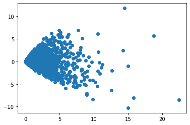
Let’s plot the first two dimensions of this vector space, so that each point is a movie:

plt.scatter(mt_P[:, 0], mt_P[:, 1])

<matplotlib.collections.PathCollection at 0x229a71673a0>

We can also plot all 5 dimensions with a pairplot. First we’re going to convert this to a data frame with named columns and a movie ID index:

mt_P_df = pd.DataFrame(mt_P, columns=[f'MD{i}' for i in range(mt_P.shape[1])], index=movies.index)
mt_P_df.head()

	MD0	MD1	MD2	MD3	MD4
movieId
1	4.975549	5.328504	5.123646	-1.189267	0.528105
2	1.403948	0.203481	1.043021	-1.659741	-0.595791
3	0.227421	0.262806	0.274965	0.162643	0.026150
4	0.144859	0.098318	-0.005974	0.057476	-0.116541
5	0.372356	0.449867	0.354281	-0.095826	0.008303

sns.pairplot(mt_P_df)

<seaborn.axisgrid.PairGrid at 0x2299e4820a0>

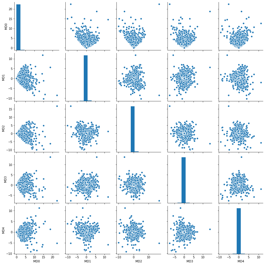
We can see that the first dimension (0) has a point that is close to a right angle; an SVD gives us orthogonal dimensions.

Now, let’s see what movies have the highest 0 dimension. Since we have a data frame, we can use nlargest:

mt_P_df.nlargest(5, 'MD0')

	MD0	MD1	MD2	MD3	MD4
movieId
260	22.462252	-8.466508	16.765136	-7.705190	-5.162488
296	18.786882	5.663466	-6.104237	13.731377	1.411248
79132	15.794102	-8.038224	-1.889724	-1.827832	5.055682
2959	15.044625	-1.071897	-9.625266	3.079433	3.910763
2571	15.021538	-10.273176	4.950140	-1.015959	3.954582

But these aren’t meaningful. Let’s join with movies to get titles:

mt_P_df.nlargest(5, 'MD0').join(movies['title'])

	MD0	MD1	MD2	MD3	MD4	title
movieId
260	22.462252	-8.466508	16.765136	-7.705190	-5.162488	Star Wars: Episode IV - A New Hope (1977)
296	18.786882	5.663466	-6.104237	13.731377	1.411248	Pulp Fiction (1994)
79132	15.794102	-8.038224	-1.889724	-1.827832	5.055682	Inception (2010)
2959	15.044625	-1.071897	-9.625266	3.079433	3.910763	Fight Club (1999)
2571	15.021538	-10.273176	4.950140	-1.015959	3.954582	Matrix, The (1999)

What about the second dimension?

mt_P_df.nlargest(5, 'MD1').join(movies['title'])

	MD0	MD1	MD2	MD3	MD4	title
movieId
356	14.526421	11.795361	1.283543	-5.822479	-5.868638	Forrest Gump (1994)
1197	7.738679	6.938436	3.866916	-1.371170	0.029446	Princess Bride, The (1987)
4306	4.914259	6.918061	4.411453	-0.466859	1.774408	Shrek (2001)
46578	5.090094	6.496026	0.156534	1.678212	3.066294	Little Miss Sunshine (2006)
4886	3.782889	6.223932	3.952054	0.045252	1.820286	Monsters, Inc. (2001)

Up to you whether you think these have a meaningful relationship.

What are the top tags for the first dimension - that is another interesting question.

I’m going to take a slightly different approach this time. I’m going to use np.argsort, which returns indexes corresponding to the sorted order of a NumPy array. The last ones will be the largest values. If I argsort a row of the mt_svd.components_ matrix, it will sort the tags by that feature; I can use the tag IDs of the highest-valued tags to get the tag names from the tag index.

Let’s go!

tag_idx[np.argsort(mt_svd.components_[0, :])[-5:]]

Index(['funny', 'based on a book', 'atmospheric', 'sci-fi', 'action'], dtype='object')

This means that movies with these tags will score highly on this feature.

Since there is a popularity component to our data (people add more tags to popular movies), there is a very good chance that the first feature will effectively be popularity.

Your Turn¶

We can also decompose the ratings matrix: users rating movies.

What are the top movies if we do that?

CS 533 Fall 2021

Movie Matrix Decomposition¶

Setup¶

Data¶

Decomposing Movie-Tags¶

Your Turn¶