Logistic Regression Demo
This notebook begins introducing the logistic regression.
Setup
Let’s import some packages:
import pandas as pd
import seaborn as sns
import numpy as np
import matplotlib.pyplot as plt
import statsmodels.api as sm
import statsmodels.formula.api as smf
rng = np.random.RandomState(20201022)
Read Data
students = pd.read_csv("https://stats.idre.ucla.edu/stat/data/binary.csv")
students.head()
| admit | gre | gpa | rank | |
|---|---|---|---|---|
| 0 | 0 | 380 | 3.61 | 3 |
| 1 | 1 | 660 | 3.67 | 3 |
| 2 | 1 | 800 | 4.00 | 1 |
| 3 | 1 | 640 | 3.19 | 4 |
| 4 | 0 | 520 | 2.93 | 4 |
Let’s train and test:
test = students.sample(frac=0.2, random_state=rng)
train_mask = pd.Series(True, index=students.index)
train_mask[test.index] = False
train = students[train_mask].copy()
train.head()
| admit | gre | gpa | rank | |
|---|---|---|---|---|
| 0 | 0 | 380 | 3.61 | 3 |
| 1 | 1 | 660 | 3.67 | 3 |
| 2 | 1 | 800 | 4.00 | 1 |
| 3 | 1 | 640 | 3.19 | 4 |
| 4 | 0 | 520 | 2.93 | 4 |
Train the Model
Now we’ll a GLM model:
mod = smf.glm('admit ~ gre + gpa + rank', train,
              family=sm.families.Binomial())
lg_res = mod.fit()
lg_res.summary()
| Dep. Variable: | admit | No. Observations: | 320 |
|---|---|---|---|
| Model: | GLM | Df Residuals: | 316 |
| Model Family: | Binomial | Df Model: | 3 |
| Link Function: | logit | Scale: | 1.0000 |
| Method: | IRLS | Log-Likelihood: | -185.53 |
| Date: | Thu, 22 Oct 2020 | Deviance: | 371.06 |
| Time: | 19:51:37 | Pearson chi2: | 321. |
| No. Iterations: | 4 | ||
| Covariance Type: | nonrobust |
| coef | std err | z | P>|z| | [0.025 | 0.975] | |
|---|---|---|---|---|---|---|
| Intercept | -3.1575 | 1.231 | -2.566 | 0.010 | -5.570 | -0.745 |
| gre | 0.0025 | 0.001 | 2.092 | 0.036 | 0.000 | 0.005 |
| gpa | 0.6554 | 0.352 | 1.862 | 0.063 | -0.035 | 1.345 |
| rank | -0.5566 | 0.141 | -3.935 | 0.000 | -0.834 | -0.279 |
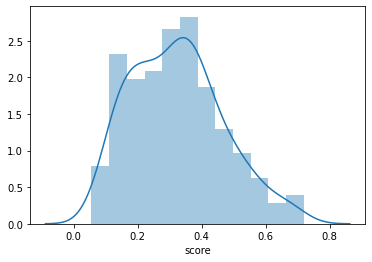
Let’s generate scores for the train data:
train['score'] = lg_res.predict(train)
sns.distplot(train['score'])
<matplotlib.axes._subplots.AxesSubplot at 0x13e4287d580>
Let’s compute the likelihood of each observed outcome:
train['like'] = train['score'].pow(train['admit'])
train['like'] *= (1 - train['score']).pow(1 - train['admit'])
train.head()
| admit | gre | gpa | rank | score | like | |
|---|---|---|---|---|---|---|
| 0 | 0 | 380 | 3.61 | 3 | 0.182807 | 0.817193 |
| 1 | 1 | 660 | 3.67 | 3 | 0.321259 | 0.321259 |
| 2 | 1 | 800 | 4.00 | 1 | 0.718391 | 0.718391 |
| 3 | 1 | 640 | 3.19 | 4 | 0.158440 | 0.158440 |
| 4 | 0 | 520 | 2.93 | 4 | 0.104835 | 0.895165 |
What is the likelhood of all the data?
train['like'].prod()
2.659838384326594e-81
That’s small! Let’s compute log likelihoods.
train['log_like'] = train['admit'] * np.log(train['score'])
train['log_like'] += (1 - train['admit']) * np.log(1 - train['score'])
train.head()
| admit | gre | gpa | rank | score | like | log_like | |
|---|---|---|---|---|---|---|---|
| 0 | 0 | 380 | 3.61 | 3 | 0.182807 | 0.817193 | -0.201880 |
| 1 | 1 | 660 | 3.67 | 3 | 0.321259 | 0.321259 | -1.135508 |
| 2 | 1 | 800 | 4.00 | 1 | 0.718391 | 0.718391 | -0.330741 |
| 3 | 1 | 640 | 3.19 | 4 | 0.158440 | 0.158440 | -1.842378 |
| 4 | 0 | 520 | 2.93 | 4 | 0.104835 | 0.895165 | -0.110747 |
Total log likelihood:
train['log_like'].sum()
-185.5311271693419
That matches the log likelihood from the GLM fit process.
What is the accuracy on the training data using 0.5 as our decision threshold:
np.mean(train['admit'] == (train['score'] > 0.5))
0.7
Analysis with Test Data
Now we’ll predict our test data:
test['score'] = lg_res.predict(test)
test.head()
| admit | gre | gpa | rank | score | |
|---|---|---|---|---|---|
| 45 | 1 | 460 | 3.45 | 3 | 0.197909 |
| 377 | 1 | 800 | 4.00 | 2 | 0.593855 |
| 322 | 0 | 500 | 3.01 | 4 | 0.104995 |
| 227 | 0 | 540 | 3.02 | 4 | 0.115585 |
| 391 | 1 | 660 | 3.88 | 2 | 0.486557 |
What are the highest-scored and lowest-scored items?
test.nlargest(5, 'score')
| admit | gre | gpa | rank | score | |
|---|---|---|---|---|---|
| 12 | 1 | 760 | 4.00 | 1 | 0.697421 |
| 69 | 0 | 800 | 3.73 | 1 | 0.681253 |
| 14 | 1 | 700 | 4.00 | 1 | 0.664381 |
| 206 | 0 | 740 | 3.54 | 1 | 0.618418 |
| 106 | 1 | 700 | 3.56 | 1 | 0.597365 |
test.nsmallest(5, 'score')
| admit | gre | gpa | rank | score | |
|---|---|---|---|---|---|
| 102 | 0 | 380 | 3.33 | 4 | 0.096431 |
| 166 | 0 | 440 | 3.24 | 4 | 0.104861 |
| 322 | 0 | 500 | 3.01 | 4 | 0.104995 |
| 179 | 0 | 300 | 3.01 | 3 | 0.109722 |
| 227 | 0 | 540 | 3.02 | 4 | 0.115585 |
Let’s make decisions with a threshold of 0.5.
test['decision'] = test['score'] > 0.5
test.head()
| admit | gre | gpa | rank | score | decision | |
|---|---|---|---|---|---|---|
| 45 | 1 | 460 | 3.45 | 3 | 0.197909 | False |
| 377 | 1 | 800 | 4.00 | 2 | 0.593855 | True |
| 322 | 0 | 500 | 3.01 | 4 | 0.104995 | False |
| 227 | 0 | 540 | 3.02 | 4 | 0.115585 | False |
| 391 | 1 | 660 | 3.88 | 2 | 0.486557 | False |
What is the accuracy of these decisions?
(test['admit'] == test['decision']).mean()
0.7375
Let’s compute the confusion matrix:
out_counts = test.groupby(['decision', 'admit'])['score'].count()
out_counts
decision  admit
False     0        52
          1        17
True      0         4
          1         7
Name: score, dtype: int64
out_counts.unstack()
| admit | 0 | 1 |
|---|---|---|
| decision | ||
| False | 52 | 17 |
| True | 4 | 7 |
What is the recall? TP / (TP + FN)
out_counts.loc[True, 1] / (out_counts.loc[True, 1] + out_counts.loc[False, 1])
0.2916666666666667
Using column/row sums:
out_counts.loc[True, 1] / out_counts.loc[:, 1].sum()
0.2916666666666667