Tuning Example
This notebook demonstrates hyperparameter tuning
It uses the CHI Papers data.
All of these are going to optimize for accuracy, the metric returned by the score function on a classifier.
Setup
scikit-optimize isn’t in Anaconda, so we’ll install it from Pip:
%pip install scikit-optimize
Requirement already satisfied: scikit-optimize in c:\users\michaelekstrand\anaconda3\lib\site-packages (0.8.1)
Requirement already satisfied: pyaml>=16.9 in c:\users\michaelekstrand\anaconda3\lib\site-packages (from scikit-optimize) (20.4.0)
Requirement already satisfied: scikit-learn>=0.20.0 in c:\users\michaelekstrand\anaconda3\lib\site-packages (from scikit-optimize) (0.23.1)
Requirement already satisfied: numpy>=1.13.3 in c:\users\michaelekstrand\anaconda3\lib\site-packages (from scikit-optimize) (1.18.5)
Requirement already satisfied: scipy>=0.19.1 in c:\users\michaelekstrand\anaconda3\lib\site-packages (from scikit-optimize) (1.5.0)
Requirement already satisfied: joblib>=0.11 in c:\users\michaelekstrand\anaconda3\lib\site-packages (from scikit-optimize) (0.16.0)
Requirement already satisfied: PyYAML in c:\users\michaelekstrand\anaconda3\lib\site-packages (from pyaml>=16.9->scikit-optimize) (5.3.1)
Requirement already satisfied: threadpoolctl>=2.0.0 in c:\users\michaelekstrand\anaconda3\lib\site-packages (from scikit-learn>=0.20.0->scikit-optimize) (2.1.0)
Note: you may need to restart the kernel to use updated packages.
Import our general PyData packages:
import pandas as pd
import numpy as np
import matplotlib.pyplot as plt
import seaborn as sns
from scipy import stats
And some SciKit Learn:
from sklearn.feature_extraction.text import TfidfVectorizer
from sklearn.decomposition import TruncatedSVD
from sklearn.neighbors import KNeighborsClassifier
from sklearn.model_selection import train_test_split, GridSearchCV, RandomizedSearchCV
from sklearn.pipeline import Pipeline
from sklearn.metrics import classification_report, accuracy_score
from sklearn.naive_bayes import MultinomialNB
And finally the Bayesian optimizer:
from skopt import BayesSearchCV
We want predictable randomness:
rng = np.random.RandomState(20201130)
In this notebook, I have SciKit-Learn run some tasks in parallel. Let’s configure the (max) number of parallel tasks in one place, so you can easily adjust it based on your computer’s capacity:
NJOBS = 8
Load Data
We’re going to load the CHI Papers data from the CSV file, output by the other notebook:
papers = pd.read_csv('chi-papers.csv', encoding='utf8')
papers.info()
<class 'pandas.core.frame.DataFrame'>
RangeIndex: 13422 entries, 0 to 13421
Data columns (total 6 columns):
 #   Column    Non-Null Count  Dtype
---  ------    --------------  -----
 0   id        13333 non-null  object
 1   title     13416 non-null  object
 2   authors   13416 non-null  object
 3   date      13422 non-null  object
 4   abstract  12926 non-null  object
 5   year      13422 non-null  int64
dtypes: int64(1), object(5)
memory usage: 629.3+ KB
Let’s treat empty abstracts as empty strings:
papers['abstract'].fillna('', inplace=True)
papers['title'].fillna('', inplace=True)
For our purposes we want all text - the title and the abstract. We will join them with a space, so we don’t fuse the last word of the title to the first word of the abstract:
papers['all_text'] = papers['title'] + ' ' + papers['abstract']
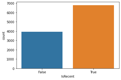
We’re going to classify papers as recent if they’re newer than 2005:
papers['IsRecent'] = papers['year'] > 2005
And make training and test data:
train, test = train_test_split(papers, test_size=0.2, random_state=rng)
Let’s make a function for measuring accuracy:
def measure(model, text='all_text'):
    preds = model.predict(test[text])
    print(classification_report(test['IsRecent'], preds))
And look at the class distribution:
sns.countplot(train['IsRecent'])
<matplotlib.axes._subplots.AxesSubplot at 0x26bb8bdde80>
Classifying New Papers
Let’s classify recent papers with k-NN on TF-IDF vectors:
base_knn = Pipeline([
    ('vectorize', TfidfVectorizer(stop_words='english', lowercase=True, max_features=10000)),
    ('class', KNeighborsClassifier(5))
])
base_knn.fit(train['all_text'], train['IsRecent'])
Pipeline(steps=[('vectorize',
                 TfidfVectorizer(max_features=10000, stop_words='english')),
                ('class', KNeighborsClassifier())])
And measure it:
measure(base_knn)
              precision    recall  f1-score   support

       False       0.39      1.00      0.56      1034
        True       0.91      0.01      0.02      1651

    accuracy                           0.39      2685
   macro avg       0.65      0.51      0.29      2685
weighted avg       0.71      0.39      0.23      2685
Tune the Neighborhood
Let’s tune the neighborhood with a grid search:
tune_knn = Pipeline([
    ('vectorize', TfidfVectorizer(stop_words='english', lowercase=True, max_features=10000)),
    ('class', GridSearchCV(KNeighborsClassifier(), param_grid={
        'n_neighbors': [1, 2, 3, 5, 7, 10]
    }, n_jobs=NJOBS))
])
tune_knn.fit(train['all_text'], train['IsRecent'])
Pipeline(steps=[('vectorize',
                 TfidfVectorizer(max_features=10000, stop_words='english')),
                ('class',
                 GridSearchCV(estimator=KNeighborsClassifier(), n_jobs=8,
                              param_grid={'n_neighbors': [1, 2, 3, 5, 7,
                                                          10]}))])
What did it pick?
tune_knn.named_steps['class'].best_params_
{'n_neighbors': 10}
And measure it:
measure(tune_knn)
              precision    recall  f1-score   support

       False       0.51      0.90      0.65      1034
        True       0.87      0.45      0.60      1651

    accuracy                           0.62      2685
   macro avg       0.69      0.67      0.62      2685
weighted avg       0.73      0.62      0.62      2685
SVD Neighborhood
Let’s set up SVD-based neighborhood, and use random search to search both the latent feature count and the neighborhood size:
svd_knn_inner = Pipeline([
    ('latent', TruncatedSVD(random_state=rng)),
    ('class', KNeighborsClassifier())
])
svd_knn = Pipeline([
    ('vectorize', TfidfVectorizer(stop_words='english', lowercase=True)),
    ('class', RandomizedSearchCV(svd_knn_inner, param_distributions={
        'latent__n_components': stats.randint(1, 50),
        'class__n_neighbors': stats.randint(1, 25)
    }, n_iter=60, n_jobs=NJOBS, random_state=rng))
])
svd_knn.fit(train['all_text'], train['IsRecent'])
Pipeline(steps=[('vectorize', TfidfVectorizer(stop_words='english')),
                ('class',
                 RandomizedSearchCV(estimator=Pipeline(steps=[('latent',
                                                               TruncatedSVD(random_state=RandomState(MT19937) at 0x26BB86DF140)),
                                                              ('class',
                                                               KNeighborsClassifier())]),
                                    n_iter=60, n_jobs=8,
                                    param_distributions={'class__n_neighbors': <scipy.stats._distn_infrastructure.rv_frozen object at 0x0000026BB8B0BEB0>,
                                                         'latent__n_components': <scipy.stats._distn_infrastructure.rv_frozen object at 0x0000026BB945A070>},
                                    random_state=RandomState(MT19937) at 0x26BB86DF140))])
What parameters did we pick?
svd_knn['class'].best_params_
{'class__n_neighbors': 21, 'latent__n_components': 21}
And measure it on the test data:
measure(svd_knn)
              precision    recall  f1-score   support

       False       0.75      0.47      0.58      1034
        True       0.73      0.90      0.81      1651

    accuracy                           0.74      2685
   macro avg       0.74      0.69      0.69      2685
weighted avg       0.74      0.74      0.72      2685
SVD with scikit-optimize
Now let’s cross-validate with SciKit-Optimize:
svd_knn_inner = Pipeline([
    ('latent', TruncatedSVD()),
    ('class', KNeighborsClassifier())
])
svd_bayes_knn = Pipeline([
    ('vectorize', TfidfVectorizer(stop_words='english', lowercase=True)),
    ('class', BayesSearchCV(svd_knn_inner, {
        'latent__n_components': (1, 50),
        'class__n_neighbors': (1, 25)
    }, n_jobs=NJOBS, random_state=rng))
])
svd_bayes_knn.fit(train['all_text'], train['IsRecent'])
C:\Users\michaelekstrand\Anaconda3\lib\site-packages\skopt\optimizer\optimizer.py:449: UserWarning: The objective has been evaluated at this point before.
  warnings.warn("The objective has been evaluated "
C:\Users\michaelekstrand\Anaconda3\lib\site-packages\skopt\optimizer\optimizer.py:449: UserWarning: The objective has been evaluated at this point before.
  warnings.warn("The objective has been evaluated "
C:\Users\michaelekstrand\Anaconda3\lib\site-packages\skopt\optimizer\optimizer.py:449: UserWarning: The objective has been evaluated at this point before.
  warnings.warn("The objective has been evaluated "
C:\Users\michaelekstrand\Anaconda3\lib\site-packages\skopt\optimizer\optimizer.py:449: UserWarning: The objective has been evaluated at this point before.
  warnings.warn("The objective has been evaluated "
C:\Users\michaelekstrand\Anaconda3\lib\site-packages\skopt\optimizer\optimizer.py:449: UserWarning: The objective has been evaluated at this point before.
  warnings.warn("The objective has been evaluated "
C:\Users\michaelekstrand\Anaconda3\lib\site-packages\skopt\optimizer\optimizer.py:449: UserWarning: The objective has been evaluated at this point before.
  warnings.warn("The objective has been evaluated "
Pipeline(steps=[('vectorize', TfidfVectorizer(stop_words='english')),
                ('class',
                 BayesSearchCV(estimator=Pipeline(steps=[('latent',
                                                          TruncatedSVD()),
                                                         ('class',
                                                          KNeighborsClassifier())]),
                               n_jobs=8,
                               random_state=RandomState(MT19937) at 0x26BB86DF140,
                               search_spaces={'class__n_neighbors': (1, 25),
                                              'latent__n_components': (1,
                                                                       50)}))])
What parameters did we pick?
svd_bayes_knn['class'].best_params_
OrderedDict([('class__n_neighbors', 25), ('latent__n_components', 20)])
And measure it:
measure(svd_bayes_knn)
              precision    recall  f1-score   support

       False       0.74      0.43      0.55      1034
        True       0.72      0.91      0.80      1651

    accuracy                           0.72      2685
   macro avg       0.73      0.67      0.67      2685
weighted avg       0.73      0.72      0.70      2685
Naive Bayes
Let’s give the Naive Bayes classifier a whirl:
nb = Pipeline([
    ('vectorize', TfidfVectorizer(stop_words='english', lowercase=True, max_features=10000)),
    ('class', MultinomialNB())
])
nb.fit(train['all_text'], train['IsRecent'])
Pipeline(steps=[('vectorize',
                 TfidfVectorizer(max_features=10000, stop_words='english')),
                ('class', MultinomialNB())])
measure(nb)
              precision    recall  f1-score   support

       False       0.89      0.50      0.64      1034
        True       0.75      0.96      0.85      1651

    accuracy                           0.78      2685
   macro avg       0.82      0.73      0.74      2685
weighted avg       0.81      0.78      0.77      2685
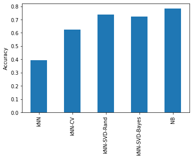
Summary Accuracy
What does our test accuracy look like for our various classifiers?
models = {
    'kNN': base_knn,
    'kNN-CV': tune_knn,
    'kNN-SVD-Rand': svd_knn,
    'kNN-SVD-Bayes': svd_bayes_knn,
    'NB': nb
}
all_preds = pd.DataFrame()
for name, model in models.items():
    all_preds[name] = model.predict(test['all_text'])
acc = all_preds.apply(lambda ds: accuracy_score(test['IsRecent'], ds))
acc
kNN              0.391806
kNN-CV           0.623836
kNN-SVD-Rand     0.735940
kNN-SVD-Bayes    0.724022
NB               0.783240
dtype: float64
acc.plot.bar()
plt.ylabel('Accuracy')
plt.show()