SciKit Transformations
This tutorial notebook demonstrates SciKit-Learn more SciKit-Learn transformations, in particular:
Using
sklearn.preprocessing.FunctionTransformerto transform two columns into oneUsing
sklearn.preprocessing.OneHotEncoderto transform a categorical column into a dummy-coded column
It builds on the ideas in the penguin regression notebook, and uses the same data.
Setup
First, we are going to import our basic packages:
import pandas as pd
import numpy as np
import matplotlib.pyplot as plt
import seaborn as sns
import scipy.stats as sps
And some SciKit-Learn code:
from sklearn.preprocessing import FunctionTransformer, OneHotEncoder, StandardScaler, PolynomialFeatures
from sklearn.compose import ColumnTransformer
from sklearn.pipeline import Pipeline
from sklearn.linear_model import LinearRegression, ElasticNetCV
from sklearn.model_selection import train_test_split
from sklearn.metrics import mean_squared_error
And initialize the RNG:
import seedbank
seedbank.initialize(20211102)
SeedSequence(
    entropy=20211102,
)
We’re going to use the Penguins data:
penguins = pd.read_csv('../data/penguins.csv')
penguins.head()
| species | island | bill_length_mm | bill_depth_mm | flipper_length_mm | body_mass_g | sex | year | |
|---|---|---|---|---|---|---|---|---|
| 0 | Adelie | Torgersen | 39.1 | 18.7 | 181.0 | 3750.0 | male | 2007 |
| 1 | Adelie | Torgersen | 39.5 | 17.4 | 186.0 | 3800.0 | female | 2007 |
| 2 | Adelie | Torgersen | 40.3 | 18.0 | 195.0 | 3250.0 | female | 2007 |
| 3 | Adelie | Torgersen | NaN | NaN | NaN | NaN | NaN | 2007 |
| 4 | Adelie | Torgersen | 36.7 | 19.3 | 193.0 | 3450.0 | female | 2007 |
Our goal is to predict penguin body mass. We’re going to remove the data where we cannot predict that:
predictable = penguins[penguins.body_mass_g.notnull()]
predictable = predictable[predictable['sex'].notnull()]
And make a train-test split:
train, test = train_test_split(predictable, test_size=0.2)
What does the training data look like?
train.head()
| species | island | bill_length_mm | bill_depth_mm | flipper_length_mm | body_mass_g | sex | year | |
|---|---|---|---|---|---|---|---|---|
| 223 | Gentoo | Biscoe | 46.4 | 15.6 | 221.0 | 5000.0 | male | 2008 |
| 273 | Gentoo | Biscoe | 50.4 | 15.7 | 222.0 | 5750.0 | male | 2009 |
| 145 | Adelie | Dream | 39.0 | 18.7 | 185.0 | 3650.0 | male | 2009 |
| 119 | Adelie | Torgersen | 41.1 | 18.6 | 189.0 | 3325.0 | male | 2009 |
| 16 | Adelie | Torgersen | 38.7 | 19.0 | 195.0 | 3450.0 | female | 2007 |
Bill Ratio
First, I would like to demonstrate how to use sklearn.preprocessing.FunctionTransformer to compute a feature from two variables: specifically, we are going to compute the bill ratio (bill length / bill depth) for each penguin.
def column_ratio(mat):
    """
    Compute the ratio of two columns.
    """
    rows, cols = mat.shape
    assert cols == 2  # if we don't have 2 columns, things are unexpected

    if hasattr(mat, 'iloc'):
        # Pandas object, use iloc
        res = mat.iloc[:, 0] / mat.iloc[:, 1]
        return res.to_frame()
    else:
        # probably a numpy array
        res = mat[:, 0] / mat[:, 1]
        return res.reshape((rows, 1))
Let’s test this on our bill columns:
column_ratio(train[['bill_length_mm', 'bill_depth_mm']])
| 0 | |
|---|---|
| 223 | 2.974359 |
| 273 | 3.210191 |
| 145 | 2.085561 |
| 119 | 2.209677 |
| 16 | 2.036842 |
| ... | ... |
| 207 | 2.922078 |
| 124 | 2.213836 |
| 200 | 3.375940 |
| 204 | 3.131944 |
| 33 | 2.164021 |
266 rows × 1 columns
Now, let’s wrap it up in a function transformer and a column transformer:
tf_br = FunctionTransformer(column_ratio)
tf_pipe = ColumnTransformer([
    ('bill_ratio', tf_br, ['bill_length_mm', 'bill_depth_mm'])
])
And apply this to our training data:
ratios = tf_pipe.fit_transform(train)
ratios[:5, :]  # first 5 rows
array([[2.97435897],
       [3.21019108],
       [2.0855615 ],
       [2.20967742],
       [2.03684211]])
That’s how you can use SciKit-Learn pipelines to combine features!
Dummy Coding
Our species and gender are categorical variables. For these we want to use dummy-coding or one-hot encoding; we specifically need the version that drops one variable, since we are doing a linear model.
We can do this with sklearn.preprocessing.OneHotEncoder. It takes an option to control dropping, and returns the encoded version of a variable.
Let’s see it in action:
enc = OneHotEncoder(drop='first')
dc = enc.fit_transform(train[['species']])
dc[:5, :].toarray()
array([[0., 1.],
       [0., 1.],
       [0., 0.],
       [0., 0.],
       [0., 0.]])
We can one-hot encode multiple categories at a single shot:
dc = enc.fit_transform(train[['species', 'sex']])
dc[:5, :].toarray()
array([[0., 1., 1.],
       [0., 1., 1.],
       [0., 0., 1.],
       [0., 0., 1.],
       [0., 0., 0.]])
We get 3 columns: 2 for the 3 levels of species, and 1 for the 2 levels of sex.
Putting It Together
Let’s now fit the model for penguins with sexual dimorphism, along with bill ratio and the excluded pairwise interactions. We’re going to do this by:
Dummy-coding species and sex
Taking the bill ratio
Standardizing flipper length
Computing all pairwise interaction terms with
sklearn.preprocessing.PolynomialFeaturesTraining a linear model, without intercepts (because the polynomial features adds a bias column)
lm_pipe = Pipeline([
    ('columns', ColumnTransformer([
        ('bill_ratio', FunctionTransformer(column_ratio), ['bill_length_mm', 'bill_depth_mm']),
        ('cats', OneHotEncoder(drop='first'), ['species', 'sex']),
        ('nums', StandardScaler(), ['flipper_length_mm']),
    ])),
    ('interact', PolynomialFeatures()),
    ('model', LinearRegression(fit_intercept=False)),
])
Now we will fit the model:
lm_pipe.fit(train, train['body_mass_g'])
Pipeline(steps=[('columns',
                 ColumnTransformer(transformers=[('bill_ratio',
                                                  FunctionTransformer(func=<function column_ratio at 0x7f4672198a60>),
                                                  ['bill_length_mm',
                                                   'bill_depth_mm']),
                                                 ('cats',
                                                  OneHotEncoder(drop='first'),
                                                  ['species', 'sex']),
                                                 ('nums', StandardScaler(),
                                                  ['flipper_length_mm'])])),
                ('interact', PolynomialFeatures()),
                ('model', LinearRegression(fit_intercept=False))])
What coefficients did this learn?
lm_pipe.named_steps['model'].coef_
array([ 5.37764531e+03, -1.16456891e+03,  3.31159495e+01, -3.23365336e+01,
       -8.40322809e+01,  7.02871964e+02,  1.39456020e+02,  1.54343148e+02,
        4.53204622e+02,  3.89303486e+02, -2.26860691e+02,  3.31159495e+01,
        2.27373675e-13, -6.81412838e+02,  2.55991981e+02, -3.23365336e+01,
       -5.95673146e+02,  2.44013269e+02, -8.40322809e+01,  9.26757085e+01,
        3.09541362e+01])
Now we can predict:
preds = lm_pipe.predict(test.drop(columns=['body_mass_g']))
mean_squared_error(test['body_mass_g'], preds)
87506.93221715576
We don’t really know how good that is without a reference point, but let’s predict mass by prediction over our test data:
sns.scatterplot(x=test['body_mass_g'], y=preds)
plt.axline((4000, 4000), slope=1, color='black')
plt.xlabel('Mass (g)')
plt.ylabel('Predicted Mass (g)')
plt.show()
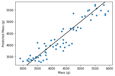
I’d say that doesn’t look too bad!
Regularization
Let’s compare that model with a regularized one.
reg_pipe = Pipeline([
    ('columns', ColumnTransformer([
        ('bill_ratio', FunctionTransformer(column_ratio), ['bill_length_mm', 'bill_depth_mm']),
        ('cats', OneHotEncoder(drop='first'), ['species', 'sex']),
        ('nums', StandardScaler(), ['flipper_length_mm']),
    ])),
    ('interact', PolynomialFeatures()),
    ('model', ElasticNetCV(l1_ratio=np.linspace(0.1, 1, 5), fit_intercept=False)),
])
Fit to our training data:
reg_pipe.fit(train, train['body_mass_g'])
Pipeline(steps=[('columns',
                 ColumnTransformer(transformers=[('bill_ratio',
                                                  FunctionTransformer(func=<function column_ratio at 0x7f4672198a60>),
                                                  ['bill_length_mm',
                                                   'bill_depth_mm']),
                                                 ('cats',
                                                  OneHotEncoder(drop='first'),
                                                  ['species', 'sex']),
                                                 ('nums', StandardScaler(),
                                                  ['flipper_length_mm'])])),
                ('interact', PolynomialFeatures()),
                ('model',
                 ElasticNetCV(fit_intercept=False,
                              l1_ratio=array([0.1  , 0.325, 0.55 , 0.775, 1.   ])))])
Let’s get curious - what L1 ratio did we learn?
reg_pipe.named_steps['model'].l1_ratio_
1.0
And what \(\alpha\) (regularization strength)?
reg_pipe.named_steps['model'].alpha_
30.840025137441792
Coefficients?
reg_pipe.named_steps['model'].coef_
array([ 940.27109261, 1213.59537801,   -0.        ,    0.        ,
          0.        ,    0.        ,  -21.53626477, -186.12301408,
         -0.        ,  228.91135821,   35.75589617,   -0.        ,
          0.        ,   -0.        ,    0.        ,    0.        ,
          0.        ,    0.        ,    0.        ,    0.        ,
          6.06733598])
Now let’s compute the prediction error:
reg_preds = reg_pipe.predict(test.drop(columns=['body_mass_g']))
mean_squared_error(test['body_mass_g'], reg_preds)
139309.94034484721
It’s worse! Not everything that is sometimes helpful is always helpful.
Conclusion
The primary purpose of this notebook was to demonstrate use of more SciKit-Learn transformation capabilities.