Overfitting Simulation
This notebook demonstrates overfitting, where we learn noise too well.
Setup
Load our modules:
import numpy as np
import pandas as pd
import seaborn as sns
import matplotlib.pyplot as plt
import statsmodels.api as sm
import statsmodels.formula.api as smf
import scipy.stats as sps
And initialize a random number generator:
rng = np.random.default_rng(20201015)
Simulating Data
Let’s define a function to generate n data points. This does three things:
Generates n samples from \(X\) uniformly at random in the range \([0,10)\) (by multiplying
randomby 10)Computes \(Y\) by \(y_i = 2 x_i + \epsilon\), where \(\epsilon \sim \mathrm{Normal}(0,2)\)
Puts \(X\) and \(Y\) into a data frame
The function:
def generate(n):
    xs = rng.random(n) * 10
    ys = xs * 2 + rng.standard_normal(n) * 2
    return pd.DataFrame({'X': xs, 'Y': ys})
Now we’re going to define a function to generate polynomials of a varible. For order \(k\), it will produce \(x^1, x^2, \dots, x^k\) as columns of a data frame:
def poly_expand(series, order=4):
    df = pd.DataFrame({'X': series})
    for i in range(2, order+1):
        df[f'X{i}'] = series ** i
    return df
Now let’s generate our initial data and plot it:
data = generate(30)
data.plot.scatter('X', 'Y')
<matplotlib.axes._subplots.AxesSubplot at 0x165d85a6160>

So far, we’ve been using StatsModels formula interface. That is syntax sugar on top of a lower-level matrix-based interface. For this analysis, we will use that, because it’s easier to programatically set up and manipulate.
The matrix interface requires us to construct an OLS instance with a \(n \times 1\) array of endogenous (outcome) variables Y, and a \(n \times k\) matrix of exogenous variables. The rows are data points, and the columns of this matrix are predictor variables. If we want an intercept, it needs to be included as a predictor variable whose value is always 1 — the sm.add_constant function does this.
Let’s set it up and fit the model:
X = sm.add_constant(data[['X']])
lin = sm.OLS(data['Y'], X)
lin = lin.fit()
lin.summary()
| Dep. Variable: | Y | R-squared: | 0.919 |
|---|---|---|---|
| Model: | OLS | Adj. R-squared: | 0.916 |
| Method: | Least Squares | F-statistic: | 317.7 |
| Date: | Fri, 16 Oct 2020 | Prob (F-statistic): | 8.13e-17 |
| Time: | 18:51:19 | Log-Likelihood: | -59.322 |
| No. Observations: | 30 | AIC: | 122.6 |
| Df Residuals: | 28 | BIC: | 125.4 |
| Df Model: | 1 | ||
| Covariance Type: | nonrobust |
| coef | std err | t | P>|t| | [0.025 | 0.975] | |
|---|---|---|---|---|---|---|
| const | -0.7818 | 0.639 | -1.223 | 0.231 | -2.091 | 0.527 |
| X | 2.2016 | 0.124 | 17.824 | 0.000 | 1.949 | 2.455 |
| Omnibus: | 7.323 | Durbin-Watson: | 1.736 |
|---|---|---|---|
| Prob(Omnibus): | 0.026 | Jarque-Bera (JB): | 5.772 |
| Skew: | 0.801 | Prob(JB): | 0.0558 |
| Kurtosis: | 4.431 | Cond. No. | 10.3 |
Warnings:
[1] Standard Errors assume that the covariance matrix of the errors is correctly specified.
Now let’s fit a 4th-order polynomial model
We’ll this by adding a constant to the poly_expand of the data frame, and fitting the model:
X = sm.add_constant(poly_expand(data['X']))
poly = sm.OLS(data['Y'], X)
poly = poly.fit()
poly.summary()
| Dep. Variable: | Y | R-squared: | 0.938 |
|---|---|---|---|
| Model: | OLS | Adj. R-squared: | 0.928 |
| Method: | Least Squares | F-statistic: | 94.82 |
| Date: | Fri, 16 Oct 2020 | Prob (F-statistic): | 9.90e-15 |
| Time: | 18:52:06 | Log-Likelihood: | -55.274 |
| No. Observations: | 30 | AIC: | 120.5 |
| Df Residuals: | 25 | BIC: | 127.6 |
| Df Model: | 4 | ||
| Covariance Type: | nonrobust |
| coef | std err | t | P>|t| | [0.025 | 0.975] | |
|---|---|---|---|---|---|---|
| const | -0.1426 | 1.135 | -0.126 | 0.901 | -2.479 | 2.194 |
| X | -1.1816 | 1.803 | -0.655 | 0.518 | -4.896 | 2.532 |
| X2 | 1.7365 | 0.805 | 2.157 | 0.041 | 0.079 | 3.394 |
| X3 | -0.2776 | 0.130 | -2.144 | 0.042 | -0.544 | -0.011 |
| X4 | 0.0138 | 0.007 | 2.027 | 0.053 | -0.000 | 0.028 |
| Omnibus: | 5.714 | Durbin-Watson: | 1.689 |
|---|---|---|---|
| Prob(Omnibus): | 0.057 | Jarque-Bera (JB): | 4.196 |
| Skew: | 0.622 | Prob(JB): | 0.123 |
| Kurtosis: | 4.345 | Cond. No. | 1.98e+04 |
Warnings:
[1] Standard Errors assume that the covariance matrix of the errors is correctly specified.
[2] The condition number is large, 1.98e+04. This might indicate that there are
strong multicollinearity or other numerical problems.
And now the same with the 10th-order polynomial:
X = sm.add_constant(poly_expand(data['X'], order=10))
poly10 = sm.OLS(data['Y'], X)
poly10 = poly10.fit()
poly10.summary()
| Dep. Variable: | Y | R-squared: | 0.946 |
|---|---|---|---|
| Model: | OLS | Adj. R-squared: | 0.918 |
| Method: | Least Squares | F-statistic: | 33.49 |
| Date: | Fri, 16 Oct 2020 | Prob (F-statistic): | 5.98e-10 |
| Time: | 18:53:18 | Log-Likelihood: | -53.154 |
| No. Observations: | 30 | AIC: | 128.3 |
| Df Residuals: | 19 | BIC: | 143.7 |
| Df Model: | 10 | ||
| Covariance Type: | nonrobust |
| coef | std err | t | P>|t| | [0.025 | 0.975] | |
|---|---|---|---|---|---|---|
| const | 0.5949 | 2.061 | 0.289 | 0.776 | -3.719 | 4.909 |
| X | -1.1089 | 19.180 | -0.058 | 0.954 | -41.254 | 39.036 |
| X2 | -18.4133 | 51.012 | -0.361 | 0.722 | -125.182 | 88.355 |
| X3 | 35.0879 | 60.911 | 0.576 | 0.571 | -92.401 | 162.577 |
| X4 | -25.8969 | 39.040 | -0.663 | 0.515 | -107.608 | 55.814 |
| X5 | 10.3116 | 14.824 | 0.696 | 0.495 | -20.715 | 41.338 |
| X6 | -2.4437 | 3.495 | -0.699 | 0.493 | -9.759 | 4.872 |
| X7 | 0.3545 | 0.517 | 0.686 | 0.501 | -0.727 | 1.436 |
| X8 | -0.0309 | 0.047 | -0.664 | 0.515 | -0.128 | 0.066 |
| X9 | 0.0015 | 0.002 | 0.636 | 0.532 | -0.003 | 0.006 |
| X10 | -3.017e-05 | 4.97e-05 | -0.607 | 0.551 | -0.000 | 7.39e-05 |
| Omnibus: | 4.482 | Durbin-Watson: | 1.745 |
|---|---|---|---|
| Prob(Omnibus): | 0.106 | Jarque-Bera (JB): | 3.177 |
| Skew: | 0.422 | Prob(JB): | 0.204 |
| Kurtosis: | 4.353 | Cond. No. | 4.80e+11 |
Warnings:
[1] Standard Errors assume that the covariance matrix of the errors is correctly specified.
[2] The condition number is large, 4.8e+11. This might indicate that there are
strong multicollinearity or other numerical problems.
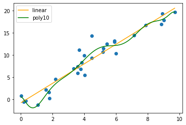
Now let’s plot the data and curves. This time, I’m going to create a linspace, as usual, and then use the fitted model’s predict function to generate the curves (this is easier than manually extracting and writing our own formula):
plt.scatter(data.X, data.Y)
xsp = np.linspace(np.min(data.X), np.max(data.X), 100)
# ysp = poly.predict(sm.add_constant(poly_expand(xsp)))
ysp10 = poly10.predict(sm.add_constant(poly_expand(xsp, order=10)))
ylp = lin.predict(sm.add_constant(xsp))
plt.plot(xsp, ylp, color='orange', label='linear')
# plt.plot(xsp, ysp, color='red', label='poly4')
plt.plot(xsp, ysp10, color='green', label='poly10')
plt.legend()
plt.show()
What are our squared errors on the training data?
np.mean(np.square(lin.resid))
3.0553433680686
np.mean(np.square(poly10.resid))
2.0253086976466195
New Data
What about new points from our distribution? Let’s generate some:
test = generate(30)
test['LinP'] = lin.predict(sm.add_constant(test[['X']]))
test['LinErr'] = test['Y'] - test['LinP']
test['Poly10P'] = poly10.predict(sm.add_constant(poly_expand(test.X, 10)))
test['Poly10Err'] = test['Y'] - test['Poly10P']
And compute our test error for each model:
np.mean(np.square(test['LinErr']))
2.992713620832882
np.mean(np.square(test['Poly10Err']))
4.382587964880173
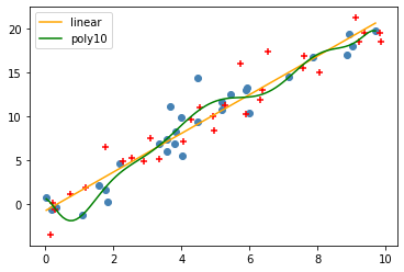
And plot the new points, along wiht the old points and our model:
plt.scatter(data.X, data.Y, color='steelblue')
plt.scatter(test.X, test.Y, color='red', marker='+')
xsp = np.linspace(np.min(data.X), np.max(data.X), 100)
# ysp = poly.predict(sm.add_constant(poly_expand(xsp)))
ysp10 = poly10.predict(sm.add_constant(poly_expand(xsp, order=10)))
ylp = lin.predict(sm.add_constant(xsp))
plt.plot(xsp, ylp, color='orange', label='linear')
# plt.plot(xsp, ysp, color='red', label='poly4')
plt.plot(xsp, ysp10, color='green', label='poly10')
plt.legend()
plt.show()