Advanced Pipeline Example
This notebook demonstrates more advanced use of SciKit-Learn pipelines; more sophisticated than my basic pipeline example and simpler than the TDS example.
The classification task is to predict whether or not a movie is an action movie. We are going to use regularized logistic regression for this task. If we can effectively predict whether a movie is an action movie from its ratings (number of ratings and/or rating values), that is evidence that action movies have different patterns than other movies; maybe they are more popular, or (on average) higher- or lower-rated.
Setup
As usual, we want to import things:
import pandas as pd
import numpy as np
import seaborn as sns
import matplotlib.pyplot as plt
And we’ll import many things from SciKit-Learn:
from sklearn.pipeline import Pipeline
from sklearn.compose import ColumnTransformer
from sklearn.preprocessing import StandardScaler, FunctionTransformer, PolynomialFeatures
from sklearn.impute import SimpleImputer
from sklearn.linear_model import LogisticRegressionCV
from sklearn.model_selection import train_test_split
And seed the RNG:
import seedbank
seedbank.initialize(20211028)
SeedSequence(
    entropy=20211028,
)
Data Preparation
Let’s first load the movie data:
movies = pd.read_csv('../data/hetrec2011-ml/movies.dat', sep='\t', encoding='latin1',
                     na_values='\\N')
movies.info()
<class 'pandas.core.frame.DataFrame'>
RangeIndex: 10197 entries, 0 to 10196
Data columns (total 21 columns):
 #   Column                  Non-Null Count  Dtype
---  ------                  --------------  -----
 0   id                      10197 non-null  int64
 1   title                   10197 non-null  object
 2   imdbID                  10197 non-null  int64
 3   spanishTitle            10197 non-null  object
 4   imdbPictureURL          10016 non-null  object
 5   year                    10197 non-null  int64
 6   rtID                    9886 non-null   object
 7   rtAllCriticsRating      9967 non-null   float64
 8   rtAllCriticsNumReviews  9967 non-null   float64
 9   rtAllCriticsNumFresh    9967 non-null   float64
 10  rtAllCriticsNumRotten   9967 non-null   float64
 11  rtAllCriticsScore       9967 non-null   float64
 12  rtTopCriticsRating      9967 non-null   float64
 13  rtTopCriticsNumReviews  9967 non-null   float64
 14  rtTopCriticsNumFresh    9967 non-null   float64
 15  rtTopCriticsNumRotten   9967 non-null   float64
 16  rtTopCriticsScore       9967 non-null   float64
 17  rtAudienceRating        9967 non-null   float64
 18  rtAudienceNumRatings    9967 non-null   float64
 19  rtAudienceScore         9967 non-null   float64
 20  rtPictureURL            9967 non-null   object
dtypes: float64(13), int64(3), object(5)
memory usage: 1.6+ MB
And we’ll need genres:
genres = pd.read_csv('../data/hetrec2011-ml/movie_genres.dat', sep='\t', encoding='latin1',
                     na_values='\\N')
genres
| movieID | genre | |
|---|---|---|
| 0 | 1 | Adventure |
| 1 | 1 | Animation |
| 2 | 1 | Children |
| 3 | 1 | Comedy |
| 4 | 1 | Fantasy |
| ... | ... | ... |
| 20804 | 65126 | Comedy |
| 20805 | 65126 | Drama |
| 20806 | 65130 | Drama |
| 20807 | 65130 | Romance |
| 20808 | 65133 | Comedy |
20809 rows × 2 columns
We’re going to get a list of action movie IDs and make our outcome column:
action_movies = genres.loc[genres['genre'] == 'Action', 'movieID']
movies['isAction'] = movies['id'].isin(action_movies)
Zero things out:
movies.loc[movies['rtAllCriticsRating'] == 0, 'rtAllCriticsRating'] = np.nan
movies.loc[movies['rtTopCriticsRating'] == 0, 'rtTopCriticsRating'] = np.nan
movies.loc[movies['rtAudienceRating'] == 0, 'rtAudienceRating'] = np.nan
Create our train/test split:
train, test = train_test_split(movies, test_size=0.25)
train.set_index('id', inplace=True)
test.set_index('id', inplace=True)
Exploration
Now that we have training data, let’s look at our class balance:
sns.countplot(x=train['isAction'])
<AxesSubplot:xlabel='isAction', ylabel='count'>
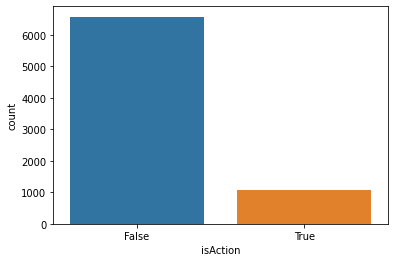
Non-action is our majority class. What is that fraction?
maj_frac = 1 - train['isAction'].mean()
maj_frac
0.8595527657905061
If our accuracy is less than 0.859, we aren’t beating majority class.
Let’s start to look at some possible correlations with our outcome variable.
rate_cols = [
    'rtAllCriticsRating', 'rtAllCriticsNumReviews',
    'rtTopCriticsRating', 'rtTopCriticsNumReviews',
    'rtAudienceRating', 'rtAudienceNumRatings'
]
pivot = train[rate_cols].melt()
pivot = pivot.join(train['isAction'])
grid = sns.FacetGrid(data=pivot, col='variable', hue='isAction', sharey=False, sharex=False)
grid.map(sns.kdeplot, 'value')
plt.show()
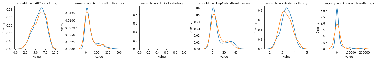
That isn’t looking promising. But the purpose of this tutorial is to demonstrate pipelines, not to build a great classifier.
Building the Classifier
For this tutorial, we are going to apply different transformations to different columns.
For average ratings, we will standardize the variables, and fill in missing values with 0 (unknown -> ignore)
For counts, we will take the log, and then standardize the logs; fill missing values with 0 (one rating)
The SciKit-Learn tool sklearn.compose.ColumnTransformer allows us to specify a transform that will do that.
SciKit-Learn doesn’t have a direct log transform, but we can use sklearn.preprocessing.FunctionTransformer with numpy.log1p().
col_ops = ColumnTransformer([
    ('ratings', Pipeline([('std', StandardScaler()), ('fill', SimpleImputer(strategy='constant', fill_value=0))]),
     ['rtAllCriticsRating', 'rtTopCriticsRating', 'rtAudienceRating']),
    ('counts', Pipeline([
        ('log', FunctionTransformer(np.log1p)),
        ('std', StandardScaler()),
        ('fill', SimpleImputer(strategy='constant', fill_value=0))]),
     ['rtAllCriticsNumReviews', 'rtTopCriticsNumReviews', 'rtAudienceNumRatings'])
])
By default, the column transformer ignores any columns that aren’t used in one of the runs. It does know enough about Pandas to use the column names.
Let’s see it in action:
col_ops.fit_transform(train)
array([[-1.42368447, -0.85740736, -1.08079972,  0.13052435,  0.43061088,
         0.89681628],
       [ 0.        ,  0.        ,  0.        , -1.4082733 , -1.28161907,
        -1.53417271],
       [ 0.54852497,  0.        ,  0.46093164, -0.53448073, -0.0274333 ,
        -0.10633124],
       ...,
       [ 0.61426528,  0.        ,  1.12167365, -0.10789001, -0.4255041 ,
         0.7642107 ],
       [-0.50332006, -0.59676893, -0.64030504,  1.42116578,  1.46636589,
         0.98862888],
       [-0.04313786,  0.        ,  0.        , -0.46530863, -1.28161907,
        -1.53417271]])
We’re also going to allow the model to use first-order interaction terms: the product of the (standardized) rating count and rating value, for example. The sklearn.preprocessing.PolynomialFeatures transformer can do that. So we will put it in a pipeline with our column operations and our final logistic regression:
lg_pipe = Pipeline([
    ('features', col_ops),
    ('interact', PolynomialFeatures()),
    ('predict', LogisticRegressionCV(penalty='l1', solver='liblinear'))
])
Now let’s fit that model:
lg_pipe.fit(train, train['isAction'])
Pipeline(steps=[('features',
                 ColumnTransformer(transformers=[('ratings',
                                                  Pipeline(steps=[('std',
                                                                   StandardScaler()),
                                                                  ('fill',
                                                                   SimpleImputer(fill_value=0,
                                                                                 strategy='constant'))]),
                                                  ['rtAllCriticsRating',
                                                   'rtTopCriticsRating',
                                                   'rtAudienceRating']),
                                                 ('counts',
                                                  Pipeline(steps=[('log',
                                                                   FunctionTransformer(func=<ufunc 'log1p'>)),
                                                                  ('std',
                                                                   StandardScaler()),
                                                                  ('fill',
                                                                   SimpleImputer(fill_value=0,
                                                                                 strategy='constant'))]),
                                                  ['rtAllCriticsNumReviews',
                                                   'rtTopCriticsNumReviews',
                                                   'rtAudienceNumRatings'])])),
                ('interact', PolynomialFeatures()),
                ('predict',
                 LogisticRegressionCV(penalty='l1', solver='liblinear'))])
How do we do on that test data?
preds = lg_pipe.predict(test)
Compute the accuracy:
np.mean(preds == test['isAction'])
0.8545098039215686
Did we just predict everything is False?
np.sum(preds)
0
Yes, yes we did. We predicted the majority class.
This classifier is not good! That happens sometimes, but we have now seen an example of a more sophisticated SciKit-Learn pipeline.